URKS Uncertainty Reasoning in Knowledge Systems
490 likes | 522 Vues
Gain insights into uncertainty in AI, probability concepts, fuzzy systems, Bayesian theory, and decision-making under uncertainty. Practical sessions included.

URKS Uncertainty Reasoning in Knowledge Systems
E N D
Presentation Transcript
URKSUncertainty Reasoningin Knowledge Systems D. Bollé H. Bruyninckx M. Nuttin D. De Schreye
Course overview: • Introduction on uncertainty in A.I. • Motivation - examples - some basic concepts • D. De Schreye (1 session) • Probability concepts, techniques and systems • Bayesian theory and approach • D. Bollé and H. Bruyninckx (+/-5 sessions) • Fuzzy concepts, techniques and systems • Zadeh theory and approach/possibility theory • M. Nuttin (+/- 6 sessions) • Comparison and question session
Practical sessions: • 5 practical (hands-on) sessions of 2.5 hours: • first: introduction to matlab • 2 sessions on probability examples • 2 sessions on fuzzy examples (second is pen-paper) • examination: exercises related to lab-sessions • (1/2 of points) • open book • remainder: written theory exam. • closed book Http://www.cs.kuleuven.ac.be/~dannyd/URKS
Introduction Uncertainty in Knowledge Systems
Levels of certainty on the uncertain probable fuzzy imprecise likely vague uncertain approximating assuming possible
Contents Contents Sources of Uncertainty. Joint probabilistic distributions. Motivating Bayes rule Utility and decision theory. Inference under uncertainty: Abductive reasoning Probabilistic reasoning GenInfer Opinion Nets Diagnosis and weak implications. Quantification types for uncertainty. What is a probability? Introducing Fuzzy sets. Prior versus Conditional probability. Probabilistic rules. Axioms of probability. Overview:
quantification of frequency with which the rule applies Sources of uncertainty: 1. Information obtained may take the form ofweak implications Ex.:in diagnosis: disease(p, Cavity) (0.8)symptom(p, Toothache) 2. Imprecise language: “often”, “sometimes”, “frequently”, “hardly ever”, … - need to quantify these in terms of frequency, - need to deal with proposed frequency in rules.
grass_is_wet sprinkler_was_on grass_is_wet rain_last_night Abductive reasoning quantification of possible conclusions quantification of measure of belief Sources of uncertainty (2): 3. Unknown information. • We observe that grass_is_wet, but have no information on sprinkler nor rain. • How to reason? • Note: can be “ranges” of unknown, depending on additional evidence. 4. Conflicting information. Ex.:Several experts have provided conflicting information:
What is Herman’s height? We may want to quantify the degree in which Herman belongs to the set of ‘tall_people’ Sources of uncertainty (3): 5. Vague Concepts: Herman is tall. - at least 1.80 m? - could Herman be 1.78 m and still tall? - if Herman is in the population of Basketball players is Herman still tall? - if Herman would be a kid of 9 years and 1.45 m is Herman also tall?
again depends on unknown information (traffic jam?, earthquake?, accident?) Quantification of estimated degree of success instead of specification of all conditions Sources of uncertainty (4): 6. Precise specifications may be too complex: Plan_90: leave 90 minutes before departure Problem: will Plan_90 succeed? BUT: enumeration of all conditions may be impossible or impractical: Succeed(Plan_90) not(car_break_down) and not(out_of_gas) and not(accident) and not(traffic_jam) and ...
Can we easily determine the uncertainty for: Tomorrow(cold) Tomorrow(rain) (?) Or for: Tomorrow(cold) Tomorrow(rain) (?) In absence of interdependencies: propagation of uncertain knowledge increases uncertainty of the conclusions Sources of uncertainty (5): 7. Propagation of uncertain information: Tomorrow(cold) (0.7) Tomorrow(rain) (0.6) Not without sufficient information on the interdependencies of the events!
Utility theory: Plan_90: leave 90 minutes before departure Plan_120: leave 120 minutes … Plan_1440: leave 24 hours ... Assume that Plan_90 is the right thing to do: whatwould this mean? Plan_120 is more likely to succeed. Plan_1440 is practically sure to succeed. BUT: Plan_90 attempts to optimize all our goals: - arrive on time for the flight - avoid long waiting at the airport - avoid getting speeding tickets for the drive - ... Utility theoryis used to represent and reason about preferences.
Decision theory: If we have expressed preferences using Utility Theory and we have expressed probabilities of events and effects by Probability Theory: Decision theory =Probability theory+Utility theory A system is rational if it chooses the action that yields the highest expected utility, averaged over all probabilities of outcomes of the action.
disease(p, Cavity) symptom(p, Toothache) symptom(p, Toothache) disease(p, Cavity) there may be other diseases ! not each cavity causes pain ! More on diagnosis andweak implications: Is it possible to capture diagnosis in hard rules ? is simply wrong disease(p, Cavity) disease(p, GumDisease) disease(p, ImpactedWisdom) … symptom(p, Toothache) Again enumeration problem: do we know them all ? wrong again There is no correct logical rule. The best we can do is provide “a quantification of belief”
Degree of belief Basic distinction Degree of membership Given Toothache, there is 80% chance of Cavity Toothache gives Cavity with factor 0.7 (in [-1,1]) Probability (respecting the axioms of probability theory) Certainty factors (don’t respect the axioms) Fuzzy Logic (measures in vague concepts) Herman is tall (with 95% measure of belonging to the set of ‘tall people’) What kind of quantifications? Degree of belief: Degree of membership:
P( randomly chosen person is Chinese) = ? all_people Chinese #(Chinese) #(all_people) = What is a probability? P(A)= number in the range [0,1] expressing the degree of belief in A. • An often used intuition: counting • Interesting intuition to verify basic axioms and rules of probability • BUT: counting is not always possible, nor desirable.
But even more often: taken as the probability Conditional probability Prior probability What is a probability? (2) • Statistics may help: • Count a randomlyselected subsetof the population • determinethe ratio(e.g.: of Chinese) from this subset • A general measure of beliefon the basis of • prior experience • intuition • ... • Crucial is: • Belief and probability changes with new gathered information !
P(A | B C) = 1/4 P(A) = 1/6 P(A | B) = 1/60 Prior versus Conditional: The Chinese student story The Bombed plane story Prior Probability: A = a randomly chosen student in some classroom is Chinese Conditional Probability: add information:B = the chosen classroom is in K.U.Leuven add information:C = the classroom is from MAI
P(A) = 1/106 P(A | A’) = 1/ 1012 P(A | B) = 1/ 106 Prior versus Conditional (2): The Bombed plane story Prior Probability: A = there is a bomb on board Conditional Probability: add information:A’ = there is (independently) another bomb on board change A’:B = I bring a second bomb myself • Prior probability (A): • probability of Ain absence of any other information • Conditional Probability (A|B): • probability of Agiven that we already knowB
P(Cavity) = 0.1 10% of all individuals have a Cavity Toothache example: P(Toothache) = 0.05 5% have a Toothache P(Cavity|Toothache) = 0.8 given that we know the individual has Toothache, there is 80% chance of him having Cavity P(Toothache|Cavity) = 0.4 conditional probability is NOT symmetric P(Cavity|Toothache not Gumdisease) = 0.9 additionally given that another diagnosis is already excluded, conditional probability increases P(Cavity|Toothache FalseTeeth) = 0 adding information does not necessarily increase the probability
A probabilistic rule A (factor)B1 B2 … Bn P(A| B1 B2 … Bn) = factor should best have the semantics: disease(p, Cavity) (0.8)symptom(p, Toothache) P(Cavity|Toothache) = 0.8 A sensible semantics for probabilistic rules: So:we simply have alternative syntax:
head [0.5,0.5] tail [0.5,0.5] A [n1,n2]B [m1,m2] head 0.0 tail In conditional probabilities semantics: But this is NOT standard at all ! In probabilistic Logic Programming (Subramanian et al.) Means:If the probability that in some possible world B is true is between m1 and m2Then the probability that in some world A is true is between n1 and n2 • Example:flip a coin, with eventsA=head,B=tail If the probability of a world in which you get tail is 0.5Then the probability of a world in which you get head is also 0.5 Notice: no world in the intersection !
A B A B The axioms of Probability 1. 0 P(A) 1 2. P(True) = 1 , P(False) = 0 3. P(A B) = P(A) + P(B) - P(A B) Derived: P(A) = 1 - P(A) Are the major difference with “certainty factor” systems: do NOT respect these axioms (Mycin: factors in range -1, 1)
Toothache Toothache 0.04 0.06 Cavity 0.01 0.89 Cavity Bayes Rule ! Joint probability distribution • Given 2 properties/events: list the entire distribution of all probability assignments to all possible combinations of truth-values for the properties/events All prior and conditional probabilities can be derived ! P(Toothache|Cavity) = 0.04 / 0.04 + 0.06 = 0.4 BUT: gathering this distribution is often not possible or at least very tedious.
burglary earthquake alarm phoneRings JohnCalls MaryCalls JohnCalls Alarm JohnCalls PhoneRings MaryCalls Alarm Loudmusic Alarm Burglary Alarm EarthQuake Inference under Uncertainty. The logic version of the burglary-alarm example: unlessLoudmusic In Logic: What can we deduce from an observation that John calls, Mary doesn’t and Mary’s CD-player was broken ?
A B A B B A B A Abductive Reasoning • Deductive reasoning:(using Modus Ponens) • Abductive reasoning:(assume A is unknown) Abducethat A holds as an explanation for the observation B • More generally:given a set of observations and a set of logical rules: find a set of hypotheses (from the unknown properties) that allow to deduce the observations
burglary earthquake alarm phoneRings unlessLoudmusic JohnCalls Alarm JohnCalls PhoneRings MaryCalls Alarm Loudmusic Alarm Burglary Alarm EarthQuake JohnCalls MaryCalls abduce deduce PhoneRings Alarm abduce abduce Burglary EarthQuake Abduction in burglar-alarm: • Unknown information : • Observation: JohnCalls • 3 possible solutions:PhoneRings Burglary EarthQuake
deduce deduce Alarm Alarm JohnCalls Alarm JohnCalls PhoneRings MaryCalls Alarm Loudmusic Alarm Burglary Alarm EarthQuake hypothesis of alarm is inconsistent with observations abduce PhoneRings Note: abductive procedures may be complicated ! Abduction in burglar-alarm (2): • Observation: JohnCalls MaryCalls LoudMusic • 1 possible explanation:PhoneRings
burglary earthquake P(E) .002 P(B) .001 alarm B E P(A) T T .95 T F .94 F T .29 F F .001 JohnCalls MaryCalls A P(J) T .90 F .05 A P(M) T .70 F .01 Acyclic directed network ! Prior probability for roots, conditional (on parents) for lower levels Belief Networks orBayesian Nets The probabilistic version of the burglary-alarm example:
burglary earthquake alarm A P(J) T .90 F .05 JohnCalls MaryCalls B E P(A) T T .95 T F .94 F T .29 F F .001 P(E) .002 P(B) .001 A P(M) T .70 F .01 Inference in Belief Networks Many (all) types of questions can be answered, using Bayes Rule. What is the probability that there is no burglary, nor earthquake, but that the alarm went and both John and Mary called? = P (J M A B E) = 0.00062 What is the probability that there is a burglary, given that John calls? = P(B | J) = ? (Bayes) 0.016
mother father Chromosomes: XX X y carrier hemophiliac child XX X y XX X y An application: GENINFER • A couple is expecting a child. • The (expecting) mother has a hemophiliac risk • determinethe probability of hemophiliacfor the child • Hemophiliac disease is genetically determined: • Due to a defected X chromosome
mother_carrier father_hemoph P(M) .00008 P(F) .00008 M F P(C) T T .75 T F .50 F T .50 F F 0 child_recessive great grandmother great grandfather C ok grandmother grandfather great uncle ? H ok A family tree: father mother ? ok ? The Bayesian Network:
GGM GGF P(GGM) 1 P(GGF) 0 P(GF) 0 P(F) 0 P(GU) 1 GM GF GU M F C Expanding to full network: Tempting solution: but these are not prior probabilities But in fact remains correct if you interpret events differently
GGM GGF P(GGM) .00008 P(F) .00008 P(GF) .00008 P(GGF) .00008 0.5 0.25 0.125 M F P(C) T T .75 T F .50 F T .50 F F 0 GM GF GU All dependencies are based on: M F C Expanding to full network (2) Compute: P(GGM| GU GGF) = 1 Compute: P(GM| GGM GGF) = 0.5 , etc.
GGM GGF GM GF GU 0.5 M U1 U2 F C 0.028 And if there are uncles? Recompute: P(GM| GMM GGF U1 U2) Propagate the information to Mother and Child
GGM GGF further decrease GM GF GU M B3 B2 B1 U1 U2 F C 0.007 And brothers? Probability under additional condition of 3 healthy bothers:
burglary earthquake JohnCalls (0.90) Alarm JohnCalls (0.05) Alarm MaryCalls (0.70) Alarm MaryCalls (0.01) Alarm Burglary (0.01) Earthquake (0.02) Alarm (0.95) Burglary Earthquake Alarm (0.94) Burglary Earthquake Alarm (0.29) Burglary Earthquake Alarm (0.001) Burglary Earthquake alarm A P(J) T .90 F .05 JohnCalls MaryCalls B E P(A) T T .95 T F .94 F T .29 F F .001 P(E) .002 P(B) .001 A P(M) T .70 F .01 Belief Networks as Rule Systems Doesn’t add anything …but shows that you need many rules to represent the full Bayesian Net In many cases you may not have all this information!
Broker 1 OR Brokers’ opinion Broker 2 AND Overall opinion Mystic 1 OR Mystic 2 Mystics’ opinion Stock_split Brokers_say_split Mystics_say_split Brokers_say_split Boker1 Broker2 Mystics_say_split Mystic1 Mystic2 Opinion Nets:when dependencies are unknown • Will the stock (on stock market) split ? • Ask the opinion of 2 brokers and of 2 mystics. + opinions (in probabilities) of Brokers and Mystics
You need upper and lower bounds! 1 Upperbound(E) P(E) Lowerbound(E) 0 Opinion Nets (2) • Problem: • We don’t know the dependencies between the opinions of the brokers and/or mystics ! • How to propagate their (probabilistic) opinions? U(E) P(E) L(E) P(E) We try to make it LeastUpperbounds and GreatestLowerbounds
… for the or connective A OR A or B B U(A) U(A or B) U(B) U(A or B) L(A) L(A or B) - U(B) L(B) L(A or B) - U(A) U(A or B) U(A) + U(B) L(A or B) max[L(A) , L(B)] Rules governing the propagation of bounds … similar for the and connective
A A B B A B B A max[P(A), P(B)] P(A or B) P(A) + P(B) max( L(A) , L(B) ) max(L(A) , L(B)) is a lowerbound for P(A or B) max(L(A) , L(B)) L(A or B) Some example inferences:
U(A or B) U(A) + U(B) OR 0.3 L(A or B) max[L(A) , L(B)] 1 0.8 0.8 1 U(A) U(A or B) 1 0.8 0.4 1 1 0 OR 0.8 0.1 0 0.4 0 0.3 1 0.3 0 0 U(B) U(A or B) 0 Propagation of opinions: Using forward propagation: Or backward propagation:
1 0.75 L(A or B) max[L(A) , L(B)] 0.25 0 OR 1 1 0.33 0.66 0 0.33 AND 1 0 0.18 = 0.33 + 0.85 -1 1 0 OR 0.15 1 0.15 0 0.85 1 0.85 L(A and B) L(A) + L(B) - 1 0 0.85 0 The global propagation (restricted to lowerbounds): • Not just Opinions: anyprobability propagation inabsence of dependenciesneeds to apply approximations.
Going Fuzzy …for a few minutes. • Examples of Fuzzy statements: • The motor is running very hot. • Tom is a very tall guy. • Electric cars are not very fast. • High-performance drives require very rapid dynamics and precise regulation. • Leuven is quite a short distance from Brussels. • Leuven is a beautiful city. • The maximum range of an electronic vehicle is short. • If short means: 300 km or less, would 301 km be long? • Want to express to what degree a property holds.
Relations: loves(John, Ann) loves(Mary, Phil) loves(Carl,Susan) Equivalent ! Sets: Functions to {0,1}: loves = {(John,Mary), (Mary, Phil), (Carl, Susan)} loves(John,Mary) = 1 loves(Mary,Phil) = 1 loves(Carl,Susan) = 1 This one allows refined statements Relations, sets and functions Offer alternative representationsof logical statements
1 1 0 0 150 150 160 160 170 170 180 180 190 190 200 200 210 210 cm cm Fuzzy sets: • Are functions: f:domain[0,1] Crisp set (tall men): Fuzzy set (tall men):
1 tall short medium 0 150 160 170 180 190 200 210 cm 1 short tall short medium 0 150 160 170 180 190 200 210 cm Representing a domain: Crisp sets (men’s height): Fuzzy set (men’s height):