
One-dimensional model
E N D
Presentation Transcript
Growth and decay of the mixed layer and seasonal thermocline from November 1989 to September 1990 at the Bermuda Atlantic Time-series Station (BATS) at 31.8°N 64.1°W. Data were collected by the Bermuda Biological Station for Research, Inc. Note that pressure in decibars is nearly the same as depth in meters (see § 6.8 for a definition of decibars).
The less stratified the water column, the greater the potential energy. It requires work to mix a stratified water column and thus increase its potential energy. The amount of energy required for complete mixing increases as the stratification increases. Much more energy is required to mix across a highly stratified thermolcine than is required in a weakly stratified deep ocean.
Strong winds at the surface can mix a stratified ocean near surface, resulting in a mixed layer. But what determines the depth of mixing?
One-dimensional model Variables are functions of z and t (1) (I=penetrating solar radiation) (2) (3) (4) b is buoyancy. Subscript r denotes constant reference state. In (2), ≈r (Boussinesq Approximation). also
Mixed layer model Assumptions: (1) The mean temperature, salinity, and horizontal velocity are assumed to be quasi-uniform within the layer (2) On the depth and time scales of the model, a quasi-discontinuous distribution can be envisaged for the same variables across the sea surface and across the lower mixed layer boundary (3) The rate at which the mean square turbulent velocity (velocity variance) changes locally is assumed small compared to the turbulence generating and dissipating effects (4) Temperature changes associated with frictional dissipation and with changes in salinity (chemical potential) are neglected
The mixed layer depth h is a new variable is mean vertical velocity (e.g., Ekman pumping) we is the rate of entrainment (water entrained from the interior below), i.e., non-turbulent to turbulent In general, when when Entrainment is associated with layer deepening. At times when the layer becomes shallower entrainment must cease.
Turbulence Kinetic Energy Equation (IV) (I) (II) (III) The rate of work by stress on the mean shear flow. As the kinetic energy of a shear flow is always larger than that of a uniform flow with the same total momentum, the reduction of mean shear by mixing generate an equivalent amount of eddy kinetic energy. The rate of work of buoyancy force (dense flow downward or light ones upward). Convergence of q and turbulent pressure fluctuation The rate of viscous dissipation of turbulence energy
Surface boundary conditions Ro surface flux of solar and terrestrial radiant energy per unit area Io surface flux of penetrating solar radiation (~45% total solar) Ho surface flux of sensible heat Qo surface flux of water vapor (evaporation) Po precipitation Ac latent heat of evaporation All fluxes are considered positive when directed upward
Bo is the rate at which buoyancy is removed from the water column (or available potential energy is supplied) by surface cooling or salinity change The mumentum fluxes boundary conditions are u* is the friction velocity. When the wind blows with a speed ua=8 m/s at a height of 10 meters about the surface, u*≈1cm/s Apart from the entrainment, the term on the right-hand-side represents a bottom drag on the mixed layer due to internal waves
Flux boundary conditions at the bottom of the mixed layer T, S, and b are the quasi-discontinuous changes of T, S, and b across the base of the mixed layer. In the absence of entrainment (we=0), all turbulent fluxes become zero at z=-h. This means that there is not enough turbulence energy available to overcome the stable stratification at the base of the layer and to produce mixing with the lower water. The mixed layer then becomes decoupled from the ocean interior.
Assume that Integrating Eq. (1) and (2) from z=0 to z=-h. To close the system, we derive we from the turbulence kinetic energy with the assumption that its production and dissipation are balanced. i.e., or
Boundary conditions for eddy kinetic energy fluxes The surface flux equals to the work by wind (multiplication of stress and wind velocity. m1 is a proportionality coefficient. The entrained (initially quiescent water) is agitated to mixed layer water by the downward turbulent energy flux. Therefore,
Given , integrating from z=0 to z=-h, we have Integrate from z=0 to an arbitrary level z above h, we have
Define Define (phase speed of internal waves at interface)
The integrated turbulence energy equation D H A B C E F G A: rate of energy needed to agitate the entrained water B: work per unit time needed to lift the dense entrained water and to mix it throughout the layer C: rate at which energy of the mean velocity field is reduced by mixing across the layer base D: rate of working by winds E: rate of potential energy change produced by fluxes across the sea surface F: rate of potential energy change produced by penetrating solar radiation G: rate of working associated with internal waves H: dissipation
It is assumed that the dissipation integral is composed of terms which are individually proportional to the active turbulence generating processes, i.e., The buoyancy generation term is non-zero only when B0 > 0 (i.e., surface cooling) Then, turbulence energy balance is In general, for h=10m
The proportional factors m, s, and n m Kato and Phillips (1969), laboratory experiments: m=1.25 Niiler and Kraus (1977): 0.6 ≤ m ≤ 4.0 Bleck (1999), OGCM results: m=1.0 Price et al. (1986), storm induced deepening: m ≤ 0.3 Davis (1981), North Pacific 20-day measurements: 0.4 ≤ m ≤ 0.5 Gasper (1988), 4-yr observations: 0.55 ≤ m ≤ 0.7 s Pollard et al., (1973): s=1 Price et al., (1986): s=0.65 n Kraus and Turner (1967): n=1 (no dissipation) Farmer (1975), mixed layer under ice: n=0.036 Gasper (1988): n=0.2
In general, these proportionality factors should not be universal constants. A scaling analysis by Niiler and Kraus (1977) shows that It is stipulated that both m and n should decrease with the layer depth h and go to zero when as h becomes very large. It means that, when the layer is too deep, all the input energy is then dissipated and non is available to increase the potential energy of the water column. This requirement may be important because, under cyclic (diurnal or seasonal) buoyancy forcing, the model with fixed m and n may not produce a totally cyclic response. The layer usually becomes deeper and potential energy increases from cycle to cycle because the continuing positive energy input by the winds (u*3 > 0)
Special Case I: Increasing stability, no wind Ro < 0, u*=0, => dh/dt < 0, we=0 (no entrainment) The energy balance becomes (surface infrared radiation heat loss) Since The layer is decoupled from the lower water. SST is increased by surface heating
Special Case II: Decreasing stability (Io=0), no wind Ro is a nonlinear function of To and atmospheric conditions. T depends not only on To but implicitly on h and temperature gradient below
Kelvin-Helmholtz Instability The perturbation system is or are finite z=0,
Assume that we have The solutions satisfying the boundary conditions at Given We have
The unstable criterion is or with D the vertical (and horizontal) scale of perturbation Let we have Bulk Richardson number
The disturbance vorticity has a phase difference with of /2
Special Case III: The effect of inertial current in the mixed layer Consider a constant wind stress is turned on at t=0 ==> Other initial conditions: Inertial current magnitude:
Any wind change generates inertial currents in the upper ocean. Their presence tends to produce a sharp velocity gradient at the layer bottom interface. When this happens, the “(C) term” in the equation below becomes important: (C) Pollard, Rhines, and Thompson (1973) argued that the shear flow generates the K-H instability when the bulk Richardson number (Ri) drops below some critical value (RiC). The finite-amplitude perturbations break up the interface and generate entrainment, causing an adjustment of layer depth to restore RiC beyond the critical value.
The turbulence energy then can be written as: For a given rate of surface forcing, a small value of the difference RiC-s must be associated with large values of we and therefore with rapid layer deepening at Also, since We have The layer reaches a maximum limiting depth hf at t=/f, one half of a pendulum day after the onset of the inertial oscillation. Inertial motion can only play an important role in the deepening process if the initial depth h(t=0) < hf
Special Case IV: deep mixed layer We define the Monin-Obukhov length L* as If h << L*, wind stirring predominates, we have If h >> L*,