Download
1 / 19
190 likes | 218 Vues
This research explores max-weight opportunistic scheduling in wireless systems using ON/OFF channels and Lyapunov functions. Analyzing N queues with 1 server, the study presents new max-weight bounds for minimizing delay. It discusses server variables, packet arrival processes, channel states, and scheduling decisions. The proposed algorithm offers advantages in throughput optimization and adaptability without the need for prior traffic rate or channel probability information. Explore approaches for improved network performance.

E N D
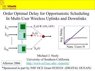
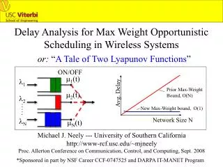
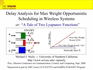
Delay Analysis for Max Weight Opportunistic Scheduling in Wireless Systems ON/OFF or: “A Tale of Two Lyapunov Functions” m1(t) l1 m2(t) l2 Prior Max-Weight Bound, O(N) Avg. Delay New Max-Weight bound, O(1) lN mN(t) Network Size N Michael J. Neely --- University of Southern California http://www-rcf.usc.edu/~mjneely Proc. Allerton Conference on Communication, Control, and Computing, Sept. 2008 *Sponsored in part by NSF Career CCF-0747525 and DARPA IT-MANET Program
Quick Description: N Queues, 1 Server, ON/OFF Channels • Slotted Time, t {0, 1, 2, 3, …}. • Ai(t) = # packets arriving to queue i on slot t (integer). • Si(t) = 0/1 Channel State (ON or OFF) for queue i on slot t. • Can serve 1 packet over a non-empty connected queue per slot. • (Scheduling: Which non-empty ON queue to serve??) ON l1 • Assume: • {Ai(t)} and {Si (t)} processes • are independent. • Ai (t) i.i.d. over slots: • E{Ai (t)} = li • Si(t) i.i.d. over slots: • Pr[Si(t) = ON] = pi ON l2 ? OFF l3 OFF l4 ON lN
Quick Description: N Queues, 1 Server, ON/OFF Channels • Slotted Time, t {0, 1, 2, 3, …}. • Ai(t) = # packets arriving to queue i on slot t (integer). • Si(t) = 0/1 Channel State (ON or OFF) for queue i on slot t. • Can serve 1 packet over a non-empty connected queue per slot. • (Scheduling: Which non-empty ON queue to serve??) OFF l1 • Assume: • {Ai(t)} and {Si (t)} processes • are independent. • Ai (t) i.i.d. over slots: • E{Ai (t)} = li • Si(t) i.i.d. over slots: • Pr[Si(t) = ON] = pi ON l2 ? OFF l3 OFF l4 ON lN
Quick Description: N Queues, 1 Server, ON/OFF Channels • Slotted Time, t {0, 1, 2, 3, …}. • Ai(t) = # packets arriving to queue i on slot t (integer). • Si(t) = 0/1 Channel State (ON or OFF) for queue i on slot t. • Can serve 1 packet over a non-empty connected queue per slot. • (Scheduling: Which non-empty ON queue to serve??) OFF l1 • Assume: • {Ai(t)} and {Si (t)} processes • are independent. • Ai (t) i.i.d. over slots: • E{Ai (t)} = li • Si(t) i.i.d. over slots: • Pr[Si(t) = ON] = pi ON l2 ? OFF l3 ON l4 ON lN
Quick Description: N Queues, 1 Server, ON/OFF Channels • Slotted Time, t {0, 1, 2, 3, …}. • Ai(t) = # packets arriving to queue i on slot t (integer). • Si(t) = 0/1 Channel State (ON or OFF) for queue i on slot t. • Can serve 1 packet over a non-empty connected queue per slot. • (Scheduling: Which non-empty ON queue to serve??) OFF l1 • Assume: • {Ai(t)} and {Si (t)} processes • are independent. • Ai (t) i.i.d. over slots: • E{Ai (t)} = li • Si(t) i.i.d. over slots: • Pr[Si(t) = ON] = pi ON l2 ? ON l3 ON l4 OFF lN
Quick Description: N Queues, 1 Server, ON/OFF Channels • Slotted Time, t {0, 1, 2, 3, …}. • Ai(t) = # packets arriving to queue i on slot t (integer). • Si(t) = 0/1 Channel State (ON or OFF) for queue i on slot t. • Can serve 1 packet over a non-empty connected queue per slot. • (Scheduling: Which non-empty ON queue to serve??) OFF l1 • Assume: • {Ai(t)} and {Si (t)} processes • are independent. • Ai (t) i.i.d. over slots: • E{Ai (t)} = li • Si(t) i.i.d. over slots: • Pr[Si(t) = ON] = pi ON l2 ? OFF l3 OFF l4 ON lN
Notation: Server variables are 0/1 variables. • Qi(t) = # packets in queue i on slot t (integer). • mi(t) = server decision (rate allocated to queue i) • = 1 if we allocate a server to queue i and Si(t) = ON. (0 else) • mi(t) = min[mi(t), Qi(t)] = actual # packets served over channel i Qi (t+1) = max[Qi(t) – mi (t), 0] + Ai (t) equivalently: Qi (t+1) = Qi(t) – mi (t) + Ai (t) l1 ? l2 Prior Max-Weight (LCQ) Bound, O(N) Avg. Delay l3 New Max-Weight (LCQ) bound, O(1) l4 Network Size N lN
Status Quo #1 – Max-Weight Scheduling: Previous Delay Bound: Capacity Region L l2 Example: r= 0.95 • N = Network Size (# of queues) • r = Fraction away from capacity • region boundary (0 < r <1) • c = constant l1 cN ≤ E{Delay} (1-r) Advantages: • Well known algorithm [Tassiulas-Ephremides 93] • Gives full throughput region (0 < r < 1). • Generalizes to multi-rate channels and multi-hop • nets with backpressure, performance opt. [NOW F&T 06] • Simple and Adaptive: No prior traffic rates or channel probabilities are required for implementation. Disadvantages: Max-Weight has no tight delay analysis!
Status Quo #2 – Queue Grouping and LCG: Largest Connected Group (LCG) Delay Bound: Capacity Region L l2 “f-balanced” region [Neely, Allerton 2006, TON 2008] l1 Delay is O(1), independent of N c log(1/(1-r)) ≤ E{Delay} (1-r) Advantages: “Largest Connected Group algorithm” (LCG)[Neely06,08] gives O(1) Average Delay, for any 0 < r < 1 in the “f-balanced region”: no individual arrival rate is more than a constant above the average rate. • More Restrictive “balanced” Throughput Region. • Requires pre-organized queue group structure based on knowledge of r and pmin = mini{Pr[Si(t)=ON]}. • Less Adaptive, not clearly connected to backpressure. Disadvantages:
Our New Results: For ON/OFF channel… • We analyze delay of Max-Weight! (use queue group concepts) • Max-Weight gives O(1) delay (anywhere in L). • We develop 2 new Lyapunov functions (“LA” & “LB”). • These tools may be useful for more general networks *(see end slide for extensions to multi-rate models). c log(1/(1-r)) c log(1/(1-r)) ≤ E{Delay} E{Delay} ≤ “f-Balanced” Rates in L Anywhere in L (1-r)2 (1-r) l2 l2 Ex: r= 0.95 Ex: r= 0.95 l1 l1 LA: LB:
Lyapunov Function 1 (LA): (ON/OFF channel) • We sum over all possible partitions of N into K disjoint groups, where K is same as in LCG algorithm: c log(1/(1-r)) E{Delay} ≤ “f-Balanced” Rates in L l1 m1(t) (1-r) l2 l2 m2(t) Ex: r= 0.95 l3 m3(t) l4 m4(t) l5 m5(t) l6 m6(t) l1 l7 m7(t) lN mN(t) LA: 0
Lyapunov Function 1 (LA): (ON/OFF channel) • We sum over all possible partitions of N into K disjoint groups, where K is same as in LCG algorithm: c log(1/(1-r)) E{Delay} ≤ “f-Balanced” Rates in L l1 m1(t) (1-r) l2 l2 m2(t) Ex: r= 0.95 l3 m3(t) l4 m4(t) l5 m5(t) l6 m6(t) l1 l7 m7(t) lN mN(t) LA: 0
Lyap. Drift DA(t) of LA(Q(t)): (ON/OFF channel) Theorem: Scheduling to minimize drift involves maximizing: where: Further, this is maximized by the Max-Weight (LCQ) Policy!
Proof Sketch: Use Combinatorics to show… Maximized by any work-conserving strategy Maximized by LCQ (“max-weight”) c1 > 0, c2 > 0
Thus: The first Lyapunov function (LA) gives: “f-Balanced” Rates in L l1 m1(t) l2 l2 m2(t) Ex: r= 0.95 l3 m3(t) c log(1/(1-r)) l4 m4(t) E{Delay} ≤ (1-r) l5 m5(t) l6 m6(t) l1 l7 m7(t) lN mN(t) LA: 0
Lyapunov Function 2 (LB): (ON/OFF channel) • A 2-part Lyapunov function, inspired by similar function in [Wu, Srikant, Perkins 2007] for different context. c log(1/(1-r)) ≤ E{Delay} Low delay when # non-empty queues is large (via multi-user diversity) (1-r)2 Stabilizes full L Anywhere in L l2 Ex: r= 0.95 LB: l1
*Extensions: (Multi-Rate Channels) • Si(t) in {0, 0.1, 0.2, …, mmax} • ***We note that this slide originally contained an incorrect claim that multi-rate channels can also achieve O(1) average delay. This claim was not in the Allerton paper, but unfortunately was in our original Arxiv pre-print (v1). We have made a new Arxiv report (v2, Dec. 08) with the corrections and discussion of issues involved: *** • M. J. Neely, “Delay Analysis for Max Weight Opportunistic Scheduling in Wireless Systems,” arXiv:0806.2345v2, Dec. 2008.
Conclusions: Order-Optimal (i.e., O(1)) Delay Analysis for the thruput-optimal Max-Weight (LCQ) Algorithm! c log(1/(1-r)) c log(1/(1-r)) ≤ E{Delay} E{Delay} ≤ “f-Balanced” Rates in L Anywhere in L (1-r)2 (1-r) l2 l2 Ex: r= 0.95 Ex: r= 0.95 • Paper:available on web: http://www-rcf.usc.edu/~mjneely/ • Extended version with the multi-rate analysis (also on web): M. J. Neely, “Delay analysis for max-weight opportunistic scheduling in wireless systems,” arXiv: 0806.2345v2, Dec. 2008. l1 l1 LA: LB:
Conclusions: Order-Optimal (i.e., O(1)) Delay Analysis for the thruput-optimal Max-Weight (LCQ) Algorithm! c log(1/(1-r)) c log(1/(1-r)) ≤ E{Delay} E{Delay} ≤ “f-Balanced” Rates in L Anywhere in L (1-r)2 (1-r) l2 l2 Ex: r= 0.95 Ex: r= 0.95 • Brief Advertisement: • Stochastic Network Optimization Homepage: http://www-rcf.usc.edu/~mjneely/stochastic/ • Contains list of papers, descriptions, other web resources, and an editable wiki board. l1 l1 LA: LB: