Download

1 / 42
420 likes | 518 Vues
Learn about phenological metrics and their interpretation using satellite imagery, compare with ground validation data, and explore different methods: thresholds, derivatives, smoothing algorithms, and model fit approaches.

E N D
Lecture 2: Modeling of Land Surface Phenology with satellite imagery Kirsten M. de Beurs, Ph.D. Assistant Professor of Geography Center for Environmental and Applied Remote Sensing (CEARS) Virginia Polytechnic Institute and State University Kdebeurs@vt.edu http://www.mapseasons.net Madison LSP Workshop: 08 APR 2008
Phenological Metrics • Phenological metrics describe the phenology of vegetation growth as observed by satellite imagery. • Standard metrics derived are: • Onset of greening • Onset of senescence • Timing of Maximum of the Growing Season • Growing season length • However, there are many more metrics available.
Maximum NDVI Rate of Senescence Rate of Greenup Time Integrated NDVI End of Season Start of Season Duration of Season SOS
Phenological Metric Phenological Interpretation • Time of SOS (EOS): beginning (end) of measurable photosynthesis. • Length of the growing season: duration of photosynthetic activity. • Time of Maximum NDVI: time of maximum photosynthesis. • NDVI at SOS (EOS): level of photosynthetic activity at SOS (EOS). • Seasonal integrated NDVI: photosynthetic activity during the growing season. • Rate of greenup (senescence): speed of increase (decrease) of photosynthesis.
Ground Validation • It is desirable to compare the satellite derived phenological estimates with data observed at ground level. • However this is not a trivial task due to: • Large pixel sizes of satellite imagery. • Composited data. • Thus, it is often unclear what LSP metrics actually track.
Four Categories: • A diversity of satellite measures and methods has been developed. • The methods can be divided into four main categories: • Threshold • Derivatives • Smoothing Algorithms • Model fit
Thresholds When do you estimate that the growing season starts?
Thresholds • Simplest method to determine SOS and EOS. • Threshold is arbitrarily set at a certain level (e.g. 0.09, 0.17, 0.3 etc). SOS EOS
Thresholds • Measure is easy to apply. • However, across the conterminous US, NDVI threshold can vary from 0.08 to 0.40. • Thus, it is inconsistent when applied towards large areas.
Thresholds based on NDVI ratios • First, translate NDVI to a ratio based on the annual minimum and maximum: NDVIratio = (NDVI-NDVImin) / (NDVImax-NDVImin)
50% is the most often used threshold. • The increase in greenness is believed to be most rapid at this threshold. • Some believe that rapid growth is more important than first leaf occurrence or bud burst. • Lower likelihood of soil – vegetation confusion than at lower thresholds.
50% Threshold (Seasonal Mid-point) (White et al., mean day = 124, May 4th)
Derivatives • What is a derivative? • What is the slope of this line? • Why?
Local Derivative Derivative is calculated based on 3 composites. (Week 3 – Week 1) / (difference in days) SOS: day where derivative is highest EOS: day where derivative is lowest
Smoothing Algorithms • Autoregressive moving average • Fourier analysis
Autoregressive moving average • Frequently used method developed in the early 1990’s by Dr. Brad Reed. • Works similarly as the thresholds method, however the threshold is established by a moving average. • What is a moving average?
Autoregressive moving average • You take the average of a certain number of time periods. • Each time period you shift one over.
Autoregressive moving average • The time lag used to calculate the forward and backward looking curves is arbitrarily chosen. • Brad Reed (1994) used a time lag of 9 composites. • In case of shorter seasons (semi-arid Africa) shorter time lags have been used (~2 months or 4 composites). Archibald and Scholes (2007).
Limitations of the moving average method • How would the moving average curve look in case of a major disturbance? • The method does not work in case of multi-peak growing seasons. • There are no clear criteria regarding the selection of the delay time.
Fourier Analysis • Fourier analysis approximates complicated curves with a sum of sinusoidal waves at multiple frequencies. • The more components are included the more the sum approximates the signal.
In phenological studies: • Amplitude: variability of productivity • Phase: measures the timing of the peak. de Beurs and Henebry, 2008
Limitations of Fourier Analysis • The Fourier composites do not necessarily have an ecological interpretation. • This approach is only useful for a study region that you know really well. • The method requires long time series, with observations that are equally spaced. • Missing values (clouds!) have to be filled. • NDVI signals are typically not exactly sinusoidal, so it is necessary to fit several terms.
Complicated adjustments High order annual splines with roughness dampening. Hermance et al. 2007
Model fit • Models based on growing degree days • Logistic Models • Gaussian Local Functions
Growing Degree Days • Development rate of plants and insects is temperature dependent. • A plant develops quicker at a higher temperature. • Daily temperature readings can be used to calculate growing degree-days • Growing degree days are a measure of accumulated heat. • Idea was first introduced in 1735 by Reaumur.
Growing Degree Days • Accumulated temperature is now recognized as the main factor influencing year-to-year variation in phenology. • Photoperiod alone, without the interaction with temperature, cannot explain the annual variability of phenology at a given location. • Photoperiod is the same in each year.
Intercept: NDVI at the start of the observed growing season. Start of Season: First composite included in the best model. NDVI peak height: NDVI at peak NDVI. Green-up period (DOY): Translated from accumulated relative humidity, the number of days necessary to reach peak NDVI • Intercept: α • Green-up period • peak position (%hum): • NDVI peak height:
Logistic Models • Straightforward logistic model • a and b are empirical coefficients that are associated with the timing and rate of change in EVI. • c+d combined give the potential maximum value • d presents the minimum value (the background EVI value). • This model can be approximated with numerical methods such as Levenberg-Marquardt Zhang, 2004
Onset_Greenness_Increase days since 1 January 2000 16-bit Onset_Greenness_Maximum days since 1 January 2000 16-bit Onset_Greenness_Decrease days since 1 January 2000 16-bit Onset_Greenness_Minimum days since 1 January 2000 16-bit NBAR_EVI_Onset_Greenness_Minimum NBAR EVI value 16-bit unsigned NBAR_EVI_Onset_Greenness_Maximum NBAR EVI value 16-bit unsigned NBAR_EVI_Area NBAR EVI area 16-bit unsigned MODIS/Terra Land Cover Dynamics Yearly L3 Global 1km SIN Grid: MOD12Q2
Gaussian Local Functions c1 and c2: base parameters determine the intercept and the amplitude of the curves, respectively. a1: the timing of the maximum (measured in time units). The upper part of the equation is fitted to the right half of the time series. The lower part of the equation fits to the left half of the time series. a2 and a4: the width of the curves a3 and a5: the flatness (or kurtosis) of the curves Jönsson and Eklundh, 2002 and Jönsson and Eklundh, 2004
Gaussian Local Functions • Applied in a program called TIMESAT
http://accweb.nascom.nasa.gov/data/ MODIS phenology for the North American Carbon Program Annual phenology data based on: • NDVI, EVI, LAI or FPAR • Spatial resolution: 250m or 500m Phenology data include: greenup date, browndown date, length of growing season, minimum NDVI, date of peak NDVI, peak NDVI, seasonal amplitude, greenup rate, browndown rate, seasonal integrated NDVI, maximum NDVI during the year, quality control map, land cover map.