Front-end, Back-end, correlators in Radiastronomy
480 likes | 765 Vues
Front-end, Back-end, correlators in Radiastronomy. Enzo Natale IRA - INAF Firenze. First MCCT-SKADS Training School September, 23-29 2007, Medicina. Topics Description of a cryo receiver - Feed horn / coupling to the antenna - Polarizer / OMT - Low Noise Amplifier

Front-end, Back-end, correlators in Radiastronomy
E N D
Presentation Transcript
Front-end, Back-end, correlators in Radiastronomy Enzo Natale IRA - INAF Firenze First MCCT-SKADS Training School September, 23-29 2007, Medicina
Topics • Description of a cryo receiver • - Feed horn / coupling to the antenna • - Polarizer / OMT • - Low Noise Amplifier • - IF processor • Receiver sensitivity • How many receiver? • - Dense focal plane array • - Array of receivers
Feed horn Trasformation from free space to guided propagation Performances Return loss : > 30 dB Insertion loss : <0.2 dB Off axis crosspol : < -35 dB Bandwidth : 30% or larger • Mode launching section(return loss - crosspol) • Flare section(taper - antenna illumination)
Optical coupling to the antenna The illumination efficiency (optical coupling) of the antenna is the ratio of the gain of the antenna to that of a uniformely illuminated aperture and is determined by the illumination function or “edge taper”, i.e. the level of the illumination at the edge of the reflector compared to that of the center. Edge taper Te = P(0) / P(re ) Te (dB) = -10 log10 (Te ) For gaussian illumination function re / w = (Te (dB) ln 10 / 20)0.5 re : reflector radius w: 1/e radius of the beam
Normalized Copolar and Crosspolar beam pattern at 22 GHz Horn for 18-26 GHz Multibeam Taper 9 dB at the edge of the subreflector (9.5°)
Multibeam horn at the Gregorian focus of SRT (simulation with GRASP by R. Nesti) Maximum gain Gi = (4 p/ l2 ) Ag Ag : geometrical area of the antenna
G/T ratio G/T = G/(TA + TR) ; TA : antenna temperature TR : receiver temperature at window Tatm = 265 K t = 0.1 f = 22 GHz
Gaussian beams To evaluate the performances achievable at the focus of a large antenna ( D >> l ) we report here some results based on the approximation of the electromagnetic field distribution in terms of Gaussian beam modes. (Goldsmith: Quasioptical System, IEEE Press, 1998). w0 waist (1/e) l wavelength r radial distance w(z) beam radius (1/e) at z z distance from the waist R curvature radius of the beam
In this approximation, it can be shown that, for not too large flare angle a a feed horn with aperture radius a and slant length R produces a gaussian beam whose waist radius is w = 0.644 a located inside the horn at a distance z approximatelye qual to 1/3 of the horn length. In these conditions about 98 % of the power radiated by the horn can be associated with the fundamental Gaussian beam mode. Using the standard formulae for Gaussian beam mode propagation , it is simple to compute the antenna illumination (the edge taper) and consequentely the full width to half maximum (FWHM) beam width in the sky of a in-focus system and unblocked aperture:
Ortho Mode Transducer (OMT) Differential Phase Shifter (DPS) The feed horn is sensitive to both linear and circular polarizations Linear polarizations are separated by the OMT Circular polarizations needs to be converted in linear (DPS)
Passive 18 - 26 GHz Front-end Feed horn Coupler DPS Waveguide to SMA converter
Turnstile junction (Navarrini, Plambeck IEEE MTT 45, Jan. 2006)
Planar OMT (Engargiola,Navarrini, IEEE MTT 53, May 2005)
Low Noise Amplifiers Typical performances of a cryogenic LNA Gain : >= 30 dB Gain flatness : ~ 1 - 2 dB Input return loss : < 15 dB Bandwidth : 30% or larger Power Out @ 1dB Compression : +5dBm Working temperature : ~ 20K Noise temperature : ~ 18 - 30 K 18 - 26 GHz ~ 30 - 50 K 36 - 50 GHz
Devices : GaAs, InP High Electron Mobility Transistors (HEMT) and Heterostructure FET (HFET) : GaAs, InP Integrated circuits 1/f noise (DG / G)2 = N A f-a N number of active devices A constant (i.e. ~ 3.6 10-8 Hz-1 for InP HEMT) a ~ 0.9 -1 (0.5!) 4 - 8 GHz 2 stages GaAs HEMT Noise T : 5K (Alma Memo 421)
LNA block diagram (inclusion of coupler + calibration source at the input?)
MMIC amplifier chip mounted Hybrid amplifier
IF Processor Receiver type : superheterodyne • IF processor • accurate definition of the receiving band • conversion of the RF band to IF band for easy interfacing to the back-end.
The mixer RF = E sin (2pnst +f) LO = V sin (2pnLOt ) I = a (RF + LO)2 = RF I • @ E2 + V2 • @ sin[2 (2pnst +f)] • @ sin [2 (2pnLOt )] • @ E V sin[2p(ns - nLO)] • @ E V sin[2p(ns + nLO)] LO I = I0 [exp(q Dv /k T ) - 1] For small Dv : I @ a (Dv)2
Receiver Sensitivity Tsys ON = Tbg + Tatm + Topt + Trec + Tsource Tsys OFF = Tbg + Tatm + Topt + Trec Tbg = 2.7 K CMB*atm Tatm = atmospheric emiss. Topt = spillover Trec = receiver Tsys ON ~ Tsys OFF s(t) = k B G Tsys If the noises are white : D Trms = Tsys (B t)-0.5 (radiometric noise)(Kraus) Tsource = Tsys ON - Tsys OFF = xs (ON source)(t) - x r (OFFsource)(t) = X(t) sX(t) = a D Trms a depends on the modulation type
But in real detecting system (receiver + atmosphere + ..) the low frequency noise is not white: • 1/fa (a ~ 1) electronics ( gain variation, ..) • 1/fa (1< a ~ 2) drift, atmosphere Power spectral density 18 - 26 GHz receiver B ~ 400 MHz t ~ 1 msec Measuring system
In this case: 1/f2 noise White noise (radiometric) 1/f noise
Allan plot 18 - 26 GHz receiver B ~ 400 MHz t ~ 1 msec White noise 1/f2 noise 1/f noise Measuring system Allan time
Mitigation of the 1/fa noise • “high” (>> 1/Allan time) modulation frequency • - ON Source / OFF Source • - On The Fly • - Two beams Dicke (equalized channels) • gain stabilization (no effect on the atmospheric noise) • - Dicke receiver ( Modulation between sky end reference source) • - Correlation receiver • - Noise injection receiver
Dicke receiver D T / Tsys = ( D G / G) (Ta - Tn )/ Tsys (Kraus, 1966) For balanced systems Ta = Tn D T / Tsys = (2 / B t)0.5
Noise injection receiver s1 = kGBTsys during toff s2 = kGB(Tsys + Tn) during ton Tsys = Tn s1/(s2 - s1) (D T/ Tsys)2 = (1/Bt) (1 + (s22 + s12)/(s2 - s1 )2 ) Tn = xTsys D T/ Tsys= (2 / Bt)0.5 (1 + 1/x + 1/x2 )0.5 W = (D T/ Tsys) / (2 / Bt)0.5 = (1 + 1/x + 1/x2 )0.5
How many receivers? Maximize observing efficiency of an antenna • Focal Plane Array • Dense FPA (mainly for n < 10 GHz) • Array of single pixel receiver
Dense array • Small array elements : about 0.5 l • Optimization of the beam properties -> high efficiecy • low spillover • Multi beam capabilities -> increase FOV • survey speed • Electronic synthesis -> flexibility • Operating frequency -> up to ~ 8GHz
PHAROS (PHased Arrays for Reflector Observing System) • Vivaldi array • 13x13 elements • pitch 21 mm • Optimized for: • prime focus 0.3-0.5 f/D • 4 - 8 GHz • Antennas, LNA, beam former cryocooled (PHAROS System Specification, Dec 2006)
Window problems : • mechanical (16 mm plexiglas) • thermal (radiation power due to the ambient ~ 45 Watt)
Array of single pixel receivers Current technology capabilities still prevent the use of dense arrays at frequencies higher than say 10 GHz. The only possibility is to build-up array by assembling together a certain number of single channel (dual polarization) receivers.. For the sake of simplicity we briefly describe the structure of an hypothetical multibeam for the 36 - 50 GHz band for Medicina antenna. Antenna: D = 32 m feq = 97 m F = feq /D = 3.04 Optical coupling efficiency : edge taper Te (dB)= 9 dB ~ 80% FWHM = (1.02 + 0.0135 Te (dB) ) l /D = 45 arcsec @ l = 7 mm Beam at primary (wa ) : 0.5 D / [Te (dB) ln(10) /20]0.5 (from the definition of edge taper) The illuminator (feed horn) must have have w0 = l feq / p wa located in the antenna focus Horn radius R = w0 /0.644 = 21.4 mm 13.8 mm ~ F l
Sampling Nyquist limit : 0.5 l F (in the focal plane) Actual sampling : 2 l F Undersampling 4 In practice + : Nyquist positions circle : horn position undersampling 5
Correction of field curvature (Petzval surface) Best focus position from the in axix focus (distance from the optical axis) Medicina antenna l = 7mm D = 500 mm
Conclusions Multi beam to increase the observing efficiency - new solutions for “simpler” front-end - integration of cal. source in the LNA - IF integration (Low cost ?) Integrated receiver (MMIC)