Segmentation Based Multi- V iew Stereo
Segmentation Based Multi- V iew Stereo. Michal Jan čošek, Tomáš Pajdla. Problem formulation : input. Input. Output. Problem formulation : output. Input. Output. Previous work. [Furukawa07] Y. Furukawa and J. Ponce. Accurate, Dense, and Robust Multi-View Stereopsis , CVPR 2007


Segmentation Based Multi- V iew Stereo
E N D
Presentation Transcript
Segmentation Based Multi-View Stereo Michal Jančošek, Tomáš Pajdla jancom1@cmp.felk.cvut.cz, pajdla@cmp.felk.cvut.cz
Problem formulation : input Input Output jancom1@cmp.felk.cvut.cz, pajdla@cmp.felk.cvut.cz
Problem formulation : output Input Output jancom1@cmp.felk.cvut.cz, pajdla@cmp.felk.cvut.cz
Previous work • [Furukawa07] Y. Furukawa and J. Ponce. Accurate, Dense, and Robust Multi-View Stereopsis, CVPR 2007 • prematching, growing, filtering • [Tao00] H. Tao and H.S. Sawhney. Global Matching Criterion and Color Segmentation Based Stereo, ACV 2000 • using segmentation for hypothesizing the continuous parts of a scene • [Felzenszwalb04] Pedro F. Felzenszwalb and Daniel P. Huttenlocher.Efficientgraph-basedimagesegmentation,IJCV2004. • color segmantation • [Jancosek08] Jancosek M. and Pajdla T. Effective seed generation for 3D reconstruction, CVWW 2008 • optimal 3D segment orientation jancom1@cmp.felk.cvut.cz, pajdla@cmp.felk.cvut.cz
Pipeline overview : Prematching Input Prematching (3D seeds) Hypothesizing (3D segments) = Output Final mesh construction Filtering (3D patches) jancom1@cmp.felk.cvut.cz, pajdla@cmp.felk.cvut.cz
Pipeline overview : 3D segments Input Prematching (3D seeds) Hypothesizing (3D segments) = Output Final mesh construction Filtering (3D patches) jancom1@cmp.felk.cvut.cz, pajdla@cmp.felk.cvut.cz
Pipeline overview : Filtering Input Prematching (3D seeds) Hypothesizing (3D segments) = Output Final mesh construction Filtering (3D patches) jancom1@cmp.felk.cvut.cz, pajdla@cmp.felk.cvut.cz
Pipeline overview : Final mesh construction Poisson Surface Reconstruction Input Prematching (3D seeds) Hypothesizing (3D segments) = Output Final mesh construction Filtering (3D patches) jancom1@cmp.felk.cvut.cz, pajdla@cmp.felk.cvut.cz
Pipeline overview : Prematching Input Prematching (3D seeds) Hypothesizing (3D segments) = Output Final mesh construction Filtering (3D patches) jancom1@cmp.felk.cvut.cz, pajdla@cmp.felk.cvut.cz
Prematching • Cameras are known (or computed [Martinec et al.]) • Feature points detection (harris on a grid [Furukawa07]) • Feature points are matched in each image pair (guided matching by epigeoms). • Matching is based on the NCC score of two 5x5 windows • Mutually best matches are selected • Tracks are constructed by grouping mutually best matches S r = ²i( ) = center of gravity of the points in S jancom1@cmp.felk.cvut.cz, pajdla@cmp.felk.cvut.cz
Pipeline overview : 3D segments Input Prematching (3D seeds) Hypothesizing (3D segments) = Output Final mesh construction Filtering (3D patches) jancom1@cmp.felk.cvut.cz, pajdla@cmp.felk.cvut.cz
3D segments • For each segment with some seed projections, we create an optimal 3D segment and set it as explored • Next we do a greedy searching of unexplored segments to explore more jancom1@cmp.felk.cvut.cz, pajdla@cmp.felk.cvut.cz
Optimal 3D segment creation TP FP TP We accept only 3D segments with the confidence above some threshold (0.6) TP – true positive FP – false positive - explored segment - unexplored segment We take only the best 3D segment according to confidence jancom1@cmp.felk.cvut.cz, pajdla@cmp.felk.cvut.cz
Optimal 3D segment creation • The goal is to find the global maximum of the criteria function Ф= 45 Ф= 75 k = 0 Ѳ= 90 Ѳ= 120 MNCC( , )= jancom1@cmp.felk.cvut.cz, pajdla@cmp.felk.cvut.cz
Optimal 3D segment creation • First, we estimate 3D segment orientation • 3D segment orientation is estimated by gradient descent optimization from the best sample out of 10x10 regular orientation samples [Jancosek08] • Next, we find the optimum position of 3D segment on the ray from reference camera center for the estimated orientation jancom1@cmp.felk.cvut.cz, pajdla@cmp.felk.cvut.cz
Greedy searching of unexplored segments TP FP TP TP TP TP – true positive FP – false positive - explored segment - unexplored segment jancom1@cmp.felk.cvut.cz, pajdla@cmp.felk.cvut.cz
Greedy searching of unexplored segments TP TP TP TP FP TP TP – true positive FP – false positive - explored segment - unexplored segment jancom1@cmp.felk.cvut.cz, pajdla@cmp.felk.cvut.cz
Pipeline overview : Filtering Input Prematching (3D seeds) Hypothesizing (3D segments) = Output Final mesh construction Filtering (3D patches) jancom1@cmp.felk.cvut.cz, pajdla@cmp.felk.cvut.cz
Filtering TP FP TP The FP 3D segments are rejected when they are not supported by another 3D segments TP – true positive FP – false positive - explored segment - unexplored segment jancom1@cmp.felk.cvut.cz, pajdla@cmp.felk.cvut.cz
Pipeline overview : Final mesh construction Poisson Surface Reconstruction Input Prematching (3D seeds) Hypothesizing (3D segments) = Output Final mesh construction Filtering (3D patches) jancom1@cmp.felk.cvut.cz, pajdla@cmp.felk.cvut.cz
Results : Strecha’s evaluation jancom1@cmp.felk.cvut.cz, pajdla@cmp.felk.cvut.cz
Results : Strecha’s evaluation jancom1@cmp.felk.cvut.cz, pajdla@cmp.felk.cvut.cz
Results : Strecha’s evaluation jancom1@cmp.felk.cvut.cz, pajdla@cmp.felk.cvut.cz
Results : Strecha’s evaluation jancom1@cmp.felk.cvut.cz, pajdla@cmp.felk.cvut.cz
Results : Strecha’s evaluation jancom1@cmp.felk.cvut.cz, pajdla@cmp.felk.cvut.cz
Results : Strecha’s evaluation jancom1@cmp.felk.cvut.cz, pajdla@cmp.felk.cvut.cz
Results : Homogenous regions jancom1@cmp.felk.cvut.cz, pajdla@cmp.felk.cvut.cz
Results : Homogenous regions jancom1@cmp.felk.cvut.cz, pajdla@cmp.felk.cvut.cz
Results : Homogenous regions jancom1@cmp.felk.cvut.cz, pajdla@cmp.felk.cvut.cz
Results : Homogenous regions jancom1@cmp.felk.cvut.cz, pajdla@cmp.felk.cvut.cz
Results : Homogenous regions jancom1@cmp.felk.cvut.cz, pajdla@cmp.felk.cvut.cz
Results : Homogenous regions jancom1@cmp.felk.cvut.cz, pajdla@cmp.felk.cvut.cz
Conclusions • Advantages • Complete models • Lack of texture is explained by planes • Speed • Possible to implement on GPU • Disadvantages • Low accuracy • Future work • MRF on volume around 3D segments jancom1@cmp.felk.cvut.cz, pajdla@cmp.felk.cvut.cz
THANK YOU FOR YOUR ATTENTION jancom1@cmp.felk.cvut.cz, pajdla@cmp.felk.cvut.cz