Download
1 / 45
450 likes | 642 Vues
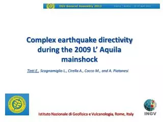
Complex earthquake directivity during the 2009 L’ Aquila mainshock. Tinti E. , Scognamiglio L., Cirella A., Cocco M., and A. Piatanesi. Istituto Nazionale di Geofisica e Vulcanologia , Rome, Italy. INTRODUCTION:. What we knew just after the 2009 L’Aquila earthquake….

E N D
Complexearthquakedirectivity during the 2009 L’ Aquila mainshock Tinti E., Scognamiglio L., Cirella A., Cocco M., and A. Piatanesi IstitutoNazionalediGeofisica e Vulcanologia, Rome, Italy
INTRODUCTION: Whatweknew just after the 2009 L’Aquila earthquake… The 2009 L’ Aquila earthquake (Mw=6.1) occurred in the CentralAppenines on April 6th at 01:32 UTC. The focal mechanism identifies a normal fault having a strike of ≈133° and a dip ≈50°.
INTRODUCTION: Whatweknew just after the 2009 L’Aquila earthquake… The 2009 L’ Aquila earthquake (Mw=6.1) occurred in the CentralAppenines on April 6th at 01:32 UTC. The focal mechanism identifies a normal fault having a strike of ≈133° and a dip ≈50°. 2) Accelerometersof RAN Network show high valuesof PGV and PGA alongsouth-east direction (seeAkinciet al 2010).
INTRODUCTION: Whatweknew just after the 2009 L’Aquila earthquake… The 2009 L’ Aquila earthquake (Mw=6.1) occurred in the CentralAppenines on April 6th at 01:32 UTC. The focal mechanism identifies a normal fault having a strike of ≈133° and a dip ≈50°. 2) Accelerometersof RAN Network show high valuesof PGV and PGA alongsouth-east direction (seeAkinciet al 2010). 3) Moment rate functionsofvelocimetershighlight a clearsouth-eastdirectivity (Pino and Di Luccio 2009).
INTRODUCTION: Whatweknew just after the 2009 L’Aquila earthquake… EP IP Accelerometerscloseto the fault show the existenceoftwoPphases: EP and IP (Di Stefano et al 2011). EP represents the ruptureonset, while IP isan impulsive phaseoccuringonly 0.9 secondsafter.
INTRODUCTION: Whatweknew just after the 2009 L’Aquila earthquake… Mainfeaturesofkinematicmodelsinferredfromnon-linearjoint inversion(Cirellaet al. 2009, 2012) are: Twomainpatches: largeralong SE, smalleralong UP DIP. Twoseparatedrupturemodes (Mode II and Mode III); High rupturevelocity in UP-DIP direction; slowerrupturepropagationalong strike. Rupture modes computed according to Pulido and Dalguer 2009 Poster XL 337; A. Cirella et al., this afternoon 17.30-19.00
MOTIVATIONS: • The 2009 L’ Aquila earthquake provided the collection of an excellent data set of seismograms and High Frequency GPS data (CGPS). We study in details the complexity of rupture process: • To unravel the directivity of this moderate magnitude earthquake; • To study the details of near source accelerograms; • To discuss the implications for ground motion prediction (engineering seismology)
RECORDED DATA: In this study we have selected the following near source data: Eight accelerograms of RAN Network and one of Mednet Network (distance < 35 km); Two continuos (High-frequency, 10Hz) GPS data: CADO and ROIO SITE EFFECTS: Because of complex geological structure, we are forced to use only frequencies lower than 0.4 Hz to exclude site effects at each station.
RECORDEDDATA: Filter: 0.02 – 0.4 Hz FN FP fault parallel FN fault normal Z vertical FP cm/s seconds
RECORDEDDATA: Filter: 0.02 – 0.4 Hz FP fault parallel FN fault normal Z vertical cm/s seconds
Fault parallel RECORDED DATA Seismograms in velocity, filtered between 0.02 – 0.4 Hz. Comparing AQU (black) and AQK (green) stations and AQV (blue) and AQG (red) stations. Fault normal Vertical AQU-AQK distance ≈500m
RECORDED DATA: POLARIGRAM Particle Motion Polarigram Horizontal Components We show the “polarigram” rather than the “particle motion” representation, because it gives at each time sample the precise amplitude and polarization of the velocity vector and makes easier a visual analysis of time series. (Bouin and Bernard,1994)
RECORDED DATA Polarigrams of filtered velocities for FN and FP components FN FP time FN FP
RECORDED DATA Arias FP fault parallel FN fault normal Z vertical
RECORDED DATA Arias high % of total energy in few seconds FP fault parallel FN fault normal Z vertical
NEW KINEMATIC INVERSION: Inversion on Finite Fault With the aimtoreproduce the detailsof the ruptureprocess, in particularof the complexdirectivity, wecompute a newkinematicmodelbyusingonlystationswithhypocentraldistancewithin 35 km and all the stationsavailable on the fault plane. Ingredients: PROCEDURE: Non-linear inversion technique (Piatanesi et al. 2007, Cirella et al 2008). VELOCITY STRUCTURE: Defined by Herrmann and Malagnini (2011). We use a L1 + L2 hybrid norm to evaluate the fit.
NEW KINEMATIC INVERSION: Inversion on Finite Fault Velocity (cm/s) synthetics data
NEW KINEMATIC INVERSION: Inversion on Finite Fault Velocity (cm/s) synthetics data
NEW KINEMATIC INVERSION: Polarigrams synthetics data
NEW KINEMATIC INVERSION: Polarigrams synthetics data
NEW KINEMATIC INVERSION: Polarigrams synthetics data
NEW KINEMATIC INVERSION: How the different patches contribute to the seismograms 0 20 0 20 0 20 synthetics data
KINEMATIC MODELING: Finite Fault Forward Modeling How the different patches contribute to the seismograms 0 20 0 20 0 20 synthetics data
KINEMATIC MODELING: Finite Fault Forward Modeling How the different patches contribute to the seismograms synthetics data 0 20 0 20 0 20 updip patch GREEN: synthetics obtained only with the along up-dip slip patch.
KINEMATIC MODELING: Finite Fault Forward Modeling How the different patches contribute to the seismograms synthetics data 0 20 0 20 0 20 updip patch GREEN: synthetics obtained only with the along up-dip slip patch.
KINEMATIC MODELING: Finite Fault Forward Modeling How the different patches contribute to the seismograms m NW SE synthetics data 0 20 0 20 0 20 along strike patch BLUE: synthetics obtained only with the along-strike slip patch.
KINEMATIC MODELING: Finite Fault Forward Modeling How the different patches contribute to the seismograms m NW SE synthetics data 0 20 0 20 0 20 along strike patch BLUE: synthetics obtained only with the along-strike slip patch.
KINEMATIC MODELING: Three forward models with: 1) homogeneous slip UPDIP (20 % of total moment) 2) constant rupture velocity (3.5-4-4.5km/s) 3) Constant rake (100°)
KINEMATIC MODELING: Three forward models with: 1) homogeneous slip UPDIP (20 % of total moment) 2) constant rupture velocity (3.5-4-4.5km/s) 3) Constant rake (100°) cm/s data
KINEMATIC MODELING: Three forward models with: 1) homogeneous slip UPDIP (20 % of total moment) 2) constant rupture velocity (3.5-4-4.5km/s) 3) Constant rake (100°) cm/s data
KINEMATIC MODELING: Three forward models with: 1) homogeneous slip UPDIP (20 % of total moment) 2) constant rupture velocity (3.5-4-4.5km/s) 3) Constant rake (100°) cm/s data UP DIP Directivity is important but more complex (GSA is overestimated with a simple model)
CONCLUSIONS: • A heterogeneous rupture process for a moderate-magnitude earthquake; • A complex directivity not revealed by initial interpretations of ground motions; • Near-fault waveforms (see AQU, AQK, AQV and AQG) mainly controlled by the UPDIP directivity, explaining the short duration of strong shaking (Arias Intensity) • Very near-source recording sites (e.g., ROIO) clearly measure the separate contributions of the two rupture propagation phases; • A detailed modeling of recorded waveforms (strong motion & HF-CGPS data) allows us to understand and demonstrate the effects of the initial fast up-dip rupture propagation, but our targeted inversion attempts do not allow us to match all the details of these waveforms • revealed by polarigrams • The rupture initially propagates at • high speed (super-shear not yet excluded) • These results have relevant implications • for near-source ground motion • prediction and GMPE
CONCLUSIONS: • A heterogeneous rupture process for a moderate-magnitude earthquake; • A complex directivity not revealed by initial interpretations of ground motions; • Near-fault waveforms (see AQU, AQK, AQV and AQG) mainly controlled by the UPDIP directivity, explaining the short duration of strong shaking (Arias Intensity) • Very near-source recording sites (e.g., ROIO) clearly measure the separate contributions of the two rupture propagation phases; • A detailed modeling of recorded waveforms (strong motion & HF-CGPS data) allows us to understand and demonstrate the effects of the initial fast up-dip rupture propagation, but our targeted inversion attempts do not allow us to match all the details of these waveforms • revealed by polarigrams • The rupture initially propagates at • high speed (super-shear not yet excluded) • These results have relevant implications • for near-source ground motion • prediction and GMPE
KINEMATIC MODELING: EVENTUALE EFFETTO DEL DIP???
Distribution of local rupture velocity reveals rupture front of Vr≈ 4km/s for the UPDIP rupture propagation
KINEMATIC MODEL: Fitting Polarigrams using Cirella et al (2012) joint inversion model ThiskinematicmodelisobtainedbyinvertingDinSar, GPS and strong motion data. Thismodeldoesn’t include AQK and AQV and ROI and CADO (CGPS). In thesestationswecompute the forwardsynthetics. synthetics data
KINEMATIC MODELING: Arias (in velocity)
RECORDED DATA FN Arias of filtered accelerograms (cumsquared acc) for near field stations:1) Few seconds 80% of total energy 2) Energy partitioned in different way FP Z FN FP
NEW KINEMATIC INVERSION: Arias. Inversion on Finite Fault Data Synthetics FP fault parallel FN fault normal Z vertical
KINEMATIC MODELING: Point Source Modeling
KINEMATIC MODELING: Point Source Modeling
KINEMATIC MODELING: Point Source Modeling