Introduction to Statistical Methods for QTL Mapping
330 likes | 421 Vues
Explore QTL mapping through lectures covering data learning, estimation techniques, and genetic concepts like allele frequencies and genotype frequencies. Understand Hardy-Weinberg equilibrium and analysis methods in biology.

Introduction to Statistical Methods for QTL Mapping
E N D
Presentation Transcript
Statistical Methods for Quantitative Trait Loci (QTL) Mapping Lectures 4 – Oct 10, 2011 CSE 527 Computational Biology, Fall 2011 Instructor: Su-In Lee TA: Christopher Miles Monday & Wednesday 12:00-1:20 Johnson Hall (JHN) 022
Outline • Learning from data • Maximum likelihood estimation (MLE) • Maximum a posteriori (MAP) • Expectation-maximization (EM) algorithm • Basic concepts • Allele, allele frequencies, genotype frequencies • Hardy-Weinberg equilibrium • Statistical methods for mapping QTL • What is QTL? • Experimental animals • Analysis of variance (marker regression) • Interval mapping (EM)
Continuous Space Revisited... • Assuming sample x1, x2,…, xn is from a mixture of parametric distributions, X x1 x2 … xm xm+1 … xn x
A Real Example • CpG content of human gene promoters GC frequency “A genome-wide analysis of CpG dinucleotides in the human genome distinguishes two distinct classes of promoters” Saxonov, Berg, and Brutlag, PNAS 2006;103:1412-1417
Mixture of Gaussians Parameters θ means variances mixing parameters P.D.F
A What-If Puzzle Likelihood • No closed form solution known for finding θ maximizing L. • However, what if we knew the hidden data?
EM as Chicken vs Egg • IF zij known, could estimate parameters θ • e.g., only points in cluster 2 influence μ2, σ2. • IF parameters θ known, could estimate zij • e.g., if |xi - μ1|/σ1 << |xi – μ2|/σ2, then zi1 >> zi2 • BUT we know neither; (optimistically) iterate: • E-step: calculate expected zij, given parameters • M-step: do “MLE” for parameters (μ,σ), given E(zij) • Overall, a clever “hill-climbing” strategy Convergence provable? YES
Simple Version: “Classification EM” • If zij < 0.5, pretend it’s 0; zij > 0.5, pretend it’s 1 i.e., classifypoints as component 0 or 1 • Now recalculate θ, assuming that partition • Then recalculate zij , assuming that θ • Then recalculate θ, assuming new zij , etc., etc.
EM summary • Fundamentally an MLE problem • EM steps • E-step: calculate expected zij, given parameters • M-step: do “MLE” for parameters (μ,σ), given E(zij) • EM is guaranteed to increase likelihood with every E-M iteration, hence will converge. • But may converge to local, not global, max. • Nevertheless, widely used, often effective
Outline • Basic concepts • Allele, allele frequencies, genotype frequencies • Hardy-Weinberg equilibrium • Statistical methods for mapping QTL • What is QTL? • Experimental animals • Analysis of variance (marker regression) • Interval mapping (Expectation Maximization)
Alleles C, G and -- are alleles …ACTCGGTTGGCCTTAATTCGGCCCGGACTCGGTTGGCCTAAATTCGGCCCGG… …ACCCGGTAGGCCTTAATTCGGCCCGGACCCGGTAGGCCTTAATTCGGCCCGG… …ACCCGGTTGGCCTTAATTCGGCCGGGACCCGGTTGGCCTTAATTCGGCCGGG… …ACTCGGTTGGCCTTAATTCGGCCCGGACTCGGTTGGCCTAAATTCGGCCCGG… …ACCCGGTAGGCCTTAATTCGGCC--GGACCCGGTAGGCCTTAATTCGGCCCGG… …ACCCGGTTGGCCTTAATTCGGCCGGGACCCGGTTGGCCTTAATTCGGCCGGG… single nucleotide polymorphism (SNP) allele frequencies for C, G, -- Alternative forms of a particular sequence Each allele has a frequency, which is the proportion of chromosomes of that type in the population
Allele frequency notations • For two alleles • Usually labeled p and q = 1 – p • e.g. p = frequency of C, q = frequency of G • For more than 2 alleles • Usually labeled pA, pB, pC... • … subscripts A, B and C indicate allele names
Genotype • The pair of alleles carried by an individual • If there are n alternative alleles … • … there will be n(n+1)/2 possible genotypes • In most cases, there are 3 possible genotypes • Homozygotes • The two alleles are in the same state • (e.g. CC, GG, AA) • Heterozygotes • The two alleles are different • (e.g. CG, AC)
Genotype frequencies Since alleles occur in pairs, these are a useful descriptor of genetic data. However, in any non-trivial study we might have a lot of frequencies to estimate. pAA, pAB, pAC,… pBB, pBC,… pCC …
The simple part • Genotype frequencies lead to allele frequencies. • For example, for two alleles: • pA = pAA + ½ pAB • pB = pBB + ½ pAB • However, the reverse is also possible!
Hardy-Weinberg Equilibrium • Relationship described in 1908 • Hardy, British mathematician • Weinberg, German physician • Shows n allele frequencies determine n(n+1)/2 genotype frequencies • Large populations • Random union of the two gametes produced by two individuals
Random Mating: Mating Type Frequencies p112 2p11p12 2p11p22 p122 2p12p22 p222 Denoting the genotype frequency of AiAj by pij,
Mendelian Segregation: Offspring Genotype Frequencies 1 0 0 p112 0.5 0.5 0 2p11p12 0 1 0 2p11p22 p122 0.25 0.5 0.25 0 0.5 0.5 2p12p22 0 0 1 p222
Required Assumptions Diploid (2 sets of DNA sequences), sexual organism Autosomal locus Large population Random mating Equal genotype frequencies among sexes Absence of natural selection
Conclusion: Hardy-Weinberg Equilibrium • Allele frequencies and genotype ratios in a randomly-breeding population remain constant from generation to generation. • Genotype frequencies are function of allele frequencies. • Equilibrium reached in one generation • Independent of initial genotype frequencies • Random mating, etc. required • Conform to binomial expansion. • (p1 + p2)2 = p12 + 2p1p2 + p22
Outline • Basic concepts • Allele, allele frequencies, genotype frequencies • Hardy-Weinberg Equilibrium • Statistical methods for mapping QTL • What is QTL? • Experimental animals • Analysis of variance (marker regression) • Interval mapping
Quantitative Trait Locus (QTL) • Definition of QTLs • The genomic regions that contribute to variation in a quantitative phenotype (e.g. blood pressure) • Mapping QTLs • Finding QTLs from data • Experimental animals • Backcross experiment (only 2 genotypes for all genes) • F2 intercross experiment
Backcross experiment parental generation first filial (F1) generation X gamete AB AA AB • Inbred strains • Homozygous genomes • Advantage • Only two genotypes • Disadvantage • Relatively less genetic diversity Karl Broman, Review of statistical methods for QTL mapping in experimental crosses
F2 intercross experiment parental generation F1 generation X F2 generation gametes AA BB AB Karl Broman, Review of statistical methods for QTL mapping in experimental crosses
QTL mapping • Data • Phenotypes: yi = trait value for mouse i • Genotypes: xik = 1/0 (i.e. AB/AA) of mouse i at marker k (backcross) • Genetic map: Locations of genetic markers • Goals • Identify the genomic regions (QTLs) contributing to variation in the phenotype. • Identify at least one QTL. • Form confidence interval for QTL location. • Estimate QTL effects.
The simplest method: ANOVA • t-test/F-statistic will tell us whether there is sufficient evidence to believe that measurements from one condition (i.e. genotype) is significantly different from another. • LOD score (“Logarithm of the odds favoring linkage”) = log10 likelihood ratio, comparing single-QTL model to the “no QTL anywhere” model. “Analysis of variance”: assumes the presence of single QTL For each marker: Split mice into groups according to their genotypes at each marker. Do a t-test/F-statistic Repeat for each typed marker
ANOVA at marker loci • Advantages • Simple. • Easily incorporate covariates (e.g. environmental factors, sex, etc). • Easily extended to more complex models. • Disadvantages • Must exclude individuals with missing genotype data. • Imperfect information about QTL location. • Suffers in low density scans. • Only considers one QTL at a time (assumes the presence of a single QTL).
Interval mapping [Lander and Botstein, 1989] • Consider any one position in the genome as the location for a putative QTL. • For a particular mouse, let z = 1/0 if (unobserved) genotype at QTL is AB/AA. • Calculate P(z = 1 | marker data). • Need only consider nearby genotyped markers. • May allow for the presence of genotypic errors. • Given genotype at the QTL, phenotype is distributed as N(µ+∆z, σ2). • Given marker data, phenotype follows a mixture of normal distributions.
IM: the mixture model Nearest flanking markers 99% AB M1/M2 65% AB 35% AA M1 QTL M2 35% AB 65% AA 0 7 20 99% AA • Let’s say that the mice with QTL genotype AA have average phenotype µA while the mice with QTL genotype AB have average phenotype µB. • The QTL has effect ∆ = µB - µA. • What are unknowns? • µA and µB • Genotype of QTL
References • Prof Goncalo Abecasis (Univ of Michigan)’s lecture note • Broman, K.W., Review of statistical methods for QTL mapping in experimental crosses • Doerge, R.W., et al. Statistical issues in the search for genes affecting quantitative traits in experimental populations. Stat. Sci.; 12:195-219, 1997. • Lynch, M. and Walsh, B. Genetics and analysis of quantitative traits. Sinauer Associates, Sunderland, MA, pp. 431-89, 1998. • Broman, K.W., Speed, T.P. A review of methods for identifying QTLs in experimental crosses, 1999.