
Programmable Logic Circuits: Computer Arithmetic: Introduction
E N D
Presentation Transcript
ELECT 90X Programmable Logic Circuits: Computer Arithmetic: Introduction Dr. Eng. Amr T. Abdel-Hamid • Slides based on slides prepared by: • B. Parhami, Computer Arithmetic: Algorithms and Hardware Design, Oxford University Press, 2000. • I. Koren, Computer Arithmetic Algorithms, 2nd Edition, A.K. Peters, Natick, MA, 2002. Fall 2009
What is Computer Arithmetic? Pentium Division Bug (1994-95): Pentium’s radix-4 SRT algorithm occasionally gave incorrect quotient First noted in 1994 by T. Nicely who computed sums of reciprocals of twin primes: 1/5 + 1/7 + 1/11 + 1/13 + . . . + 1/p + 1/(p + 2) + . . . Worst-case example of division error in Pentium:
A Motivating Example Using a calculator with √, x2, and xy functions, compute: u = √√ … √ 2= 1.000 677 131 “1024th root of 2” v = 21/1024 = 1.000 677 131 Save u and v; If you can’t save, recompute values when needed x = (((u2)2)...)2 = 1.999 999 963 x' = u1024 = 1.999 999 973 y = (((v2)2)...)2 = 1.999 999 983 y' = v1024 = 1.999 999 994 Perhaps v and u are not really the same value w = v – u = 1 10–11 Nonzero due to hidden digits (u – 1) 1000 =0.677 130 680 [Hidden ... (0) 68] (v – 1) 1000 =0.677 130 690 [Hidden ... (0) 69]
Finite Range Can Lead to Disaster Example: Explosion of Ariane Rocket (1996 June 4) Unmanned Ariane 5 rocket of the European Space Agency veered off its flight path, broke up, and exploded only 30 s after lift-off (altitude of 3700 m) The $500 million rocket (with cargo) was on its first voyage after a decade of development costing $7 billion Cause: “software error in the inertial reference system” Problem specifics: A 64 bit floating point number relating to the horizontal velocity of the rocket was being converted to a 16 bit signed integer An SRI* software exception arose during conversion because the 64-bit floating point number had a value greater than what could be represented by a 16-bit signed integer (max 32 767) *SRI = Inertial Reference System
Encoding Numbers in 4 Bits Some of the possible ways of assigning 16 distinct codes to represent numbers.
The Binary Number System • In conventional digital computers - integers represented as binary numbers of fixed length n • An ordered sequence of binary digits • Each digit x (bit) is 0 or 1 • The above sequence represents the integer value X • Upper case letters represent numerical values or sequences of digits • Lower case letters, usually indexed, represent individual digits i
Radix of a Number System • The weight of the digit x is the i th power of 2 • 2 is the radix of the binary number system • Binary numbers are radix-2 numbers - allowed digits are 0,1 • Decimal numbers are radix-10 numbers - allowed digits are 0,1,2,…,9 • Radix indicated in subscript as a decimal number • Example: • (101) - decimal value 101 • (101) - decimal value 5 i 10 2
Range of Representations • Operands and results are stored in registers of fixed length n - finite number of distinct values that can be represented within an arithmetic unit • Xmin ; Xmax - smallest and largest representable values • [Xmin,Xmax] - range of the representable numbers • A result larger then Xmax or smaller than Xmin - incorrectly represented • The arithmetic unit should indicate that the generated result is in error - an overflowindication
Example - Overflow in Binary System • Unsigned integers with 5 binary digits (bits) • Xmax = (31)10 - represented by (11111)2 • Xmin = (0)10 - represented by (00000)2 • Increasing Xmax by 1 = (32)10 =(100000)2 • 5-bit representation - only the last five digits retained - yielding (00000)2 =(0)10 • In general - • A number X not in the range [Xmin,Xmax]=[0,31] is represented by X mod 32 • If X+Y exceeds Xmax - the result is S = (X+Y) mod 32 • Example: X 10001 17 +Y 10010 18 1 00011 3 = 35 mod 32 • Result has to be stored in a 5-bit register - the most significant bit (with weight 2 =32) is discarded 5
Fixed Radix Systems • r - the radix of the number system • Conventional number systems are also called fixed-radix systems • With no redundancy - 0 xi r-1 • xi r introduces redundancy into the fixed-radix number system ?? HOW? • If xi r is allowed - • two machine representations for the same value -(...,xi+1,xi,... ) and (...,xi+1+1,xi-r,... )
Representation of Mixed Numbers • A sequence of n digits in a register - not necessarily representing an integer • Can represent a mixed number with a fractional part and an integral part • The n digits are partitioned into two - k in the integral part and m in the fractional part (k+m=n) • The value of an n-tuple with a radix point between the k most significant digits and the m least significant digits • is
Fixed Point Representations • Radix point not stored in register - understood to be in a fixed position between the k most significant digits and the m least significant digits • These are called fixed-point representations • Programmer not restricted to the predetermined position of the radix point • Operands can be scaled - same scaling for all operands • Add and subtract operations are correct - • aX aY=a(X Y) (a - scaling factor) • Corrections required for multiplication and division • aX aY=a X Y ; aX/aY=X/Y • Commonly used positions for the radix point - • rightmost side of the number (pure integers - m=0) • leftmost side of the number (pure fractions - k=0) 2
ULP - Unit in Last Position • Given the length n of the operands, the weight r of the least significant digit indicates the position of the radix point • Unit in the last position (ulp) - the weight of the least significant digit • ulp = r • This notation simplifies the discussion • No need to distinguish between the different partitions of numbers into fractional and integral parts -m -m
Representation of Negative Numbers • Fixed-point numbers in a radix r system • Two ways of representing negative numbers: • Sign and magnituderepresentation (or signed-magnitude representation) • Complement representation with two alternatives • Radix complement (two's complement in the binary system) • Diminished-radix complement (one's complement in the binary system)
Signed-Magnitude Representation • Sign and magnitude are represented separately • First digit is the sign digit, remaining n-1 digits represent the magnitude • Binary case - sign bit is 0 for positive, 1 for negative numbers • Non-binary case - 0 and r-1 indicate positive and negative numbers • Only 2r out of the r possible sequences are utilized • Two representations for zero - positive and negative • Inconvenient when implementing an arithmetic unit - when testing for zero, the two different representations must be checked n-1 n
Disadvantage of the Signed-Magnitude Representation • Operation may depend on the signs of the operands • Example - adding a positive number X and a negative number -Y : X+(-Y) • If Y>X, final result is -(Y-X) • Calculation - • switch order of operands • perform subtraction rather than addition • attach the minus sign • A sequence of decisions must be made, costing excess control logic and execution time • This is avoided in the complement representation methods
Complement Representations of Negative Numbers • Two alternatives - • Radix complement (called two's complement in the binary system) • Diminished-radix complement (called one's complement in the binary system) • In both complement methods - positive numbers represented as in the signed-magnitude method • A negative number -Y is represented by R-Y where R is a constant • This representation satisfies -(-Y )=Y since R-(R-Y)=Y
Advantage of Complement Representation • No decisions made before executing addition or subtraction • Example: X-Y=X+(-Y) • -Y is represented by R-Y • Addition is performed by X+(R-Y) = R-(Y-X) • If Y>X, -(Y-X) is already represented as R-(Y-X) • No need to interchange the order of the two operands
Two’s Complement 0 • r=2, k=n=4, m=0, ulp=2 =1 • Radix complement (called two's complement in the binary case) of a number X = 2 - X • It can instead be calculated by X+1 • 0000 to 0111 represent positive numbers 010 to 710 • The two's complement of 0111 is 1000+1=1001 • it represents the value (-7)10 • The two's complement of 0000 is 1111+1=10000=0 mod 2 - single representation of zero • Each positive number has a corresponding negative number that starts with a 1 • 1000 representing (-8)10 has no corresponding positive number • Range of representable numbers is -8 X 7 4 - 4
Example - Addition in Two’s complement • Calculating X+(-Y) with Y>X - 3+(-5) 0011 3 + 1011 -5 1110 -2 • Correct result represented in the two's complement method - no need for preliminary decisions or post corrections • Calculating X+(-Y) with X>Y - 5+(-3) 0101 5 + 1101 -3 1 0010 2 • Only the last four least significant digits are retained, yielding 0010
One’s Complement in Binary System • r=2, k=n=4, m=0, ulp=2 =1 • Diminished-radix complement (called one's complement in the binary case) of a number X = (2 - 1) - X = X • As before, the sequences 0000 to 0111 represent the positive numbers 010 to 710 • The one's complement of 0111 is 1000, representing (-7)10 • The one's complement of zero is 1111 - two representations of zero • Range of representable numbers is -7 X 7 0 4 -
5.1 Bit-Serial and Ripple-Carry Adders Half-adder (HA): Truth table and block diagram Full-adder (FA): Truth table and block diagram
Half-Adder Implementations c Three implementations of a half-adder.
Full-Adder Implementations Possible designs for a full-adder in terms of half-adders, logic gates, and CMOS transmission gates.
Full-Adder Details Logic equations for a full-adder: s = xycin (odd parity function) = xycinxycinxycinxycin cout = x yx ciny cin (majority function) CMOS transmission gate and its use in a 2-to-1 mux.
Simple Adders Built of Full-Adders Using full-adders in building bit-serial and ripple-carry adders.
Critical Path Through a Ripple-Carry Adder Tripple-add = TFA(x,ycout) + (k – 2)TFA(cincout) + TFA(cins) Critical path in a k-bit ripple-carry adder.
Binary Adders as Versatile Building Blocks Set one input to 0: cout = AND of other inputs Set one input to 1: cout = OR of other inputs Set one input to 0 and another to 1: s = NOT of third input Four-bit binary adder used to realize the logic function f = w + xyz and its complement.
Conditions and Exceptions Two’s-complement adder with provisions for detecting conditions and exceptions. overflow2’s-compl = ckck–1 = ckck–1ck ck–1
Manchester Carry Chains and Adders Sum digit in radix rsi =(xi + yi + ci) mod r Special case of radix 2 si =xiyici Computing the carries ci is thus our central problem For this, the actual operand digits are not important What matters is whether in a given position a carry is generated, propagated, or annihilated (absorbed) For binary addition: gi = xi yipi = xiyiai =xiyi = (xiyi) It is also helpful to define a transfer signal: ti = gipi = ai= xiyi Using these signals, the carry recurrence is written as ci+1= gici pi = gici gici pi = gici ti
Carry Network is the Essence of a Fast Adder gi = xiyi pi = xiyi Ripple; Skip; Lookahead; Parallel-prefix The main part of an adder is the carry network. The rest is just a set of gates to produce the g and p signals and the sum bits.
Ripple-Carry Adder Revisited The carry recurrence: ci+1 = gipici Latency of k-bit adder is roughly 2k gate delays: 1 gate delay for production of p and g signals, plus 2(k – 1) gate delays for carry propagation, plus 1 XOR gate delay for generation of the sum bits The carry propagation network of a ripple-carry adder.
The Complete Design of a Ripple-Carry Adder gi = xiyi pi = xiyi
Unrolling the Carry Recurrence Recall the generate, propagate, annihilate (absorb), and transfer signals: SignalRadix rBinary gi is 1 iff xi + yirxi yi pi is 1 iff xi + yi = r – 1xiyi ai is 1 iff xi + yi < r – 1xiyi = (xiyi) ti is 1 iff xi + yir – 1 xiyi si (xi + yi + ci) mod rxiyici The carry recurrence can be unrolled to obtain each carry signal directly from inputs, rather than through propagation ci = gi–1ci–1pi–1 = gi–1 (gi–2ci–2pi–2)pi–1 = gi–1gi–2pi–1ci–2pi–2pi–1 = gi–1gi–2pi–1gi–3pi–2pi–1ci–3pi–3pi–2pi–1 = gi–1gi–2pi–1gi–3pi–2pi–1gi–4pi–3pi–2pi–1ci–4pi–4pi–3pi–2pi–1 = . . .
Full Carry Lookahead x3 y3 x2 y2 x1 y1 x0 y0 cin . . . s3 s2 s1 s0 Theoretically, it is possible to derive each sum digit directly from the inputs that affect it Carry-lookahead adder design is simply a way of reducing the complexity of this ideal, but impractical, arrangement by hardware sharing among the various lookahead circuits
Four-Bit Carry-Lookahead Adder Complexity reduced by deriving the carry-out indirectly Four-bit carry network with full lookahead. Full carry lookahead is quite practical for a 4-bit adder c1= g0c0p0 c2= g1g0p1c0p0p1 c3= g2g1p2g0p1p2c0p0p1p2 c4= g3g2p3g1p2p3g0p1p2p3 c0p0p1p2p3
Carry Lookahead Beyond 4 Bits . . . 32-input OR Consider a 32-bit adder c1= g0c0p0 c2= g1g0p1c0p0p1 c3= g2g1p2g0p1p2c0p0p1p2 . . . c31= g30g29p30g28p29p30g27p28p29p30 . . . c0p0p1p2p3...p29p30 32-input AND High fan-ins necessitate tree-structured circuits
Solutions to the Fan-in Problem • Multilevel lookahead • Block Adders • High-radix addition (i.e., radix 2h) : Increases the latency for generating g and p signals and sum digits, but simplifies the carry network (optimal radix?) • Example: 16-bit addition • Radix-16 (four digits) • Two-level carry lookahead (four 4-bit blocks) • Either way, the carries c4, c8, and c12 are determined first • c16 c15 c14 c13 c12 c11 c10 c9 c8c7c6c5c4c3c2c1c0 • Cout ? ? ? cin
Larger Carry-Lookahead Adder Design • Block generate and propagate signals • g[i,i+3]= gi+3gi+2pi+3gi+1pi+2pi+3gi pi+1pi+2pi+3 • p[i,i+3]= pi pi+1pi+2pi+3 • If all 4 bits in a block propagate, the block propagates a carry. • If at least one of the 4 bits generates carry and it can be propagated to the MSB, the block generates a carry.
A Building Block for Carry-Lookahead Addition Four-bit lookahead carry generator. Four-bit adder
Combining Block g and p Signals Combining of g and p signals of four blocks of arbitrary widths into the g and p signals for the overall block
A Two-Level Carry-Lookahead Adder Building a 64-bit carry-lookahead adder from 16 4-bit adders and 5 lookahead carry generators.
Ling Adder and Related Designs Consider the carry recurrence and its unrolling by 4 steps: ci = gi–1ci–1ti–1 = gi–1gi–2ti–1gi–3ti–2ti–1gi–4ti–3ti–2ti–1ci–4ti–4ti–3ti–2ti–1 Ling’s modification: Propagate hi = cici–1 instead of ci hi = gi–1hi–1ti–2 = gi–1gi–2gi–3ti–2gi–4ti–3ti–2hi–4ti–4ti–3ti–2 CLA: 5 gates max 5 inputs 19 gate inputs Ling: 4 gates max 5 inputs 14 gate inputs The advantage of hi over ci is even greater with wired-OR: CLA: 4 gates max 5 inputs 14 gate inputs Ling: 3 gates max 4 inputs 9 gate inputs Once hi is known, however, the sum is obtained by a slightly more complex expression compared with si = pici si= (tihi+1) hi gi ti–1
Formulating the Prefix Computation Problem The problem of carry determination can be formulated as: Given (g0, p0) (g1, p1) . . . (gk–2, pk–2) (gk–1, pk–1) Find (g[0,0] , p[0,0]) (g[0,1] , p[0,1]) . . . (g[0,k–2] , p[0,k–2]) (g[0,k–1] , p[0,k–1]) c1c2 . . . ck–1ck The desired pairs are found by evaluating all prefixes of (g0, p0) ¢ (g1, p1) ¢ . . . ¢ (gk–2, pk–2) ¢ (gk–1, pk–1) The carry operator ¢ is associative, but not commutative [(g1, p1) ¢ (g2, p2)] ¢ (g3, p3) = (g1, p1) ¢ [(g2, p2) ¢ (g3, p3)] Prefix sums analogy: Given x0x1x2 . . . xk–1 Find x0x0+x1x0+x1+x2 . . . x0+x1+...+xk–1
Example Prefix-Based Carry Network 6 2 -1 5 12 6 7 5 ¢ ¢ ¢ ¢ g3, p3 g3, p3 g2, p2 g2, p2 g1, p1 g1, p1 g0, p0 g0, p0 g[0,3], p[0,3] =(c4, --) g[0,3], p[0,3] =(c4, --) g[0,2], p[0,2] =(c3, --) g[0,2], p[0,2] =(c3, --) g[0,1], p[0,1] =(c2, --) g[0,1], p[0,1] =(c2, --) g[0,0], p[0,0] =(c1, --) g[0,0], p[0,0] =(c1, --) + + Four-input prefix sums network + + Scan order Four-bit Carry lookahead network
Alternative Parallel Prefix Networks Parallel prefix sums network built of two k/2-input networks and k/2 adders. (Ladner-Fischer)