Chapter 12 Kinematics
Chapter 12 Kinematics. ME 242 Chapter 12. Question 1 We obtain the acceleration fastest By taking the derivative of x(t) By Integrating x(t) twice By integrating the accel as function of displacement By computing the time to liftoff, then choosing the accel such that the velocity is 160 mph.

Chapter 12 Kinematics
E N D
Presentation Transcript
ME 242 Chapter 12 • Question 1 We obtain the acceleration fastest • By taking the derivative of x(t) • By Integrating x(t) twice • By integrating the accel as function of displacement • By computing the time to liftoff, then choosing the accel such that the velocity is 160 mph
160 mi/h = 235 ft/s ME 242 Chapter 12 • Question 2 The acceleration is approximately • 92 ft/s2 • 66 ft/s2 • 85.3 ft/s2 • 182 ft/s2 • 18.75 ft/s2 Ya pili
ME 242 Chapter 12 Solution: 160 mi/h = 235 ft/s We use v*dv = a*dx Integrate:1/2v2 = a*d, where d is the length of the runway, and the start velocity = 0 • Question 2 The acceleration is approximately • 92 ft/s2 • 66 ft/s2 • 85.3 ft/s2 • 182 ft/s2 • 18.75 ft/s2 Ya kwanza
Question 3Road map: We obtain the velocity fastest • By Taking the derivative of a(t) • By Integrating a(t) • By integrating the accel as function of displacement • By computing the time to bottom, then computing the velocity.
ME242 Tutoring • Graduate Assistant Ms. Yang Liu will be available to assist with homework preparation and answer questions. • Coordination through the Academic Success Center in TBE-A 207 Tuesday and Friday mornings. • Contact hours: MW after class
ME242 Reading Assignments • Look up the next Homework assignment on Mastering • Example: your second assignment covers sections 12.5 and 12.6 • Study the text and practice the examples in the book • An I-Clicker reading test on each chapter section will be given at the start of each lecture • More time for discussion and examples
Supplemental Instruction ME 242 • Questions • Yang Liu – PhD student in ME • yangliu205@gmail.com • Lab: SEB 4261
Chapter 12-5 Curvilinear Motion X-Y Coordinates
NORMAL AND TANGENTIAL COMPONENTS (Section 12.7) When a particle moves along a curved path, it is sometimes convenient to describe its motion using coordinates other than Cartesian. When the path of motion is known, normal(n) and tangential(t)coordinates are often used. In the n-t coordinate system, the origin is located ontheparticle (the origin moves with the particle). The t-axis is tangent to the path (curve) at the instant considered, positive in the direction of the particle’s motion. The n-axis is perpendicular to the t-axis with the positive direction toward the center of curvature of the curve.
NORMAL AND TANGENTIAL COMPONENTS (continued) The positive n and t directions are defined by the unit vectorsun and ut, respectively. The center of curvature, O’, always lies on the concave side of the curve. The radius of curvature, r, is defined as the perpendicular distance from the curve to the center of curvature at that point. The position of the particle at any instant is defined by the distance, s, along the curve from a fixed reference point.
Acceleration is the time rate of change of velocity: a = dv/dt = d(vut)/dt = vut + vut . . . Here v represents the change in the magnitude of velocity and ut represents the rate of change in the direction of ut. . After mathematical manipulation, the acceleration vector can be expressed as: . a = vut + (v2/r) un = at ut + an un. ACCELERATION IN THE n-t COORDINATE SYSTEM
• The tangential component is tangent to the curve and in the direction of increasing or decreasing velocity. at = v or at ds = v dv . ACCELERATION IN THE n-t COORDINATE SYSTEM (continued) So, there are two components to the acceleration vector: a = at ut + an un • The normal or centripetal component is always directed toward the center of curvature of the curve. an = v2/r • The magnitude of the acceleration vector is a = [(at)2 + (an)2]0.5
NORMAL AND TANGENTIAL COMPONENTS (Section 12.7) When a particle moves along a curved path, it is sometimes convenient to describe its motion using coordinates other than Cartesian. When the path of motion is known, normal(n) and tangential(t)coordinates are often used. In the n-t coordinate system, the origin is located ontheparticle (the origin moves with the particle). The t-axis is tangent to the path (curve) at the instant considered, positive in the direction of the particle’s motion. The n-axis is perpendicular to the t-axis with the positive direction toward the center of curvature of the curve.
Normal and Tangential Coordinates Velocity Page 53
Normal and Tangential Coordinates ‘e’ denotes unit vector (‘u’ in Hibbeler)
‘e’ denotes unit vector (‘u’ in Hibbeler)
Learning Techniques • Complete Every Homework • Team with fellow students • Study the Examples • Ask: Ms. Yang, peers, me • Mathcad provides structure and numerically correct results
Course Concepts • Math • Think Conceptually • Map your approach BEFORE starting work
Polar coordinates ‘e’ denotes unit vector (‘u’ in Hibbeler)
Polar coordinates ‘e’ denotes unit vector (‘u’ in Hibbeler)
. . .
. . .
. . .
12.10 Relative (Constrained) Motion vA is given as shown. Find vB Approach: Use rel. Velocity: vB = vA +vB/A (transl. + rot.)
Vectors and Geometry r(t) y q q(t) x
12.10 Relative (Constrained) Motion V_truck = 60 V_car = 65 Make a sketch: A V_rel v_Truck B • The rel. velocity is: • V_Car/Truck = v_Car -vTruck
Example Vector equation: Sailboat tacking at 50 deg. against Northern Wind (blue vector) We solve Graphically (Vector Addition)
Example Vector equation: Sailboat tacking at 50 deg. against Northern Wind An observer on land (fixed Cartesian Reference) sees Vwind and vBoat . Land
12.10 Relative (Constrained) Motion Plane Vector Addition is two-dimensional. vA vB vB/A
Example cont’d: Sailboat tacking against Northern Wind 2. Vector equation (1 scalar eqn. each in i- and j-direction). Solve using the given data (Vector Lengths and orientations) and Trigonometry 500 150 i
Exam 1 • We will focus on Conceptual Solutions. Numbers are secondary. • Train the General Method • Topics: All covered sections of Chapter 12 • Practice: Train yourself to solve all Problems in Chapter 12
Exam 1 Preparation: Start now! Cramming won’t work. Questions: Discuss with your peers. Ask me. The exam will MEASURE your knowledge and give you objective feedback.
Exam 1 Preparation: Practice: Step 1: Describe Problem Mathematically Step2: Calculus and Algebraic Equation Solving
And here a few visual observations about contemporary forms of socializing, sent to me by a colleague at the Air Force Academy. Enjoy!