Using R in Astronomy
This document presents various applications of R in astronomy, focusing on graphical visualizations and data analysis. Dr. Juan Pablo Torres-Papaqui from the University of Guanajuato exemplifies R's powerful plotting capabilities through an array of plots, such as Planck blackbody curves, boxplots, and spatial distributions of galaxies. Each example is accompanied by R code for reproducibility, showcasing how to generate informative and visually appealing graphics relevant to astronomical data. This serves as a valuable resource for astronomers and researchers employing statistical analysis in their work.

Using R in Astronomy
E N D
Presentation Transcript
Using R in Astronomy Examples Dr. Juan Pablo Torres-Papaqui Departamento de Astronomía Universidad de Guanajuato DA-UG, México papaqui@astro.ugto.mx División de Ciencias Naturales y Exactas, Campus Guanajuato, Sede Valenciana
R has great graphics and plotting capabilities and can produce a wide range of plots very easily. The following is an R plot gallery with a selection of different R plot types and graphs that were all generated with R. In each case you can click on the graph to see the commented code that produced the plot in R. Note that the R code produces pdf files, which I have converted in gimp to png format for displaying on the web.
Planck Blackbody curves
#--Define blackbody function: blackbody <- function(lambda, Temp=1e3) { h <- 6.626068e-34; c <- 3e8; kb <- 1.3806503e-23 # constants lambda <- lambda * 1e-6 # Convert from metres to microns ( 2*pi*h*c^2 ) / ( lambda^5*( exp( (h*c)/(lambda*kb*Temp) ) - 1 ) ) }
#--Define title and axis labels: main <- "Planck blackbody curves" xlab <- expression(paste(Wavelength, " (", mu, "m)")) ylab <- expression(paste(Intensity, " ", (W/m^3))) #--Line styles and colours: ## (see colorbrewer2.org) ## require(RColorBrewer) ## col <- brewer.pal(3, "Dark2") col <- c("#1B9E77", "#D95F02", "#7570B3") lty <- 1:3 # Line type lwd <- 2.5 # Line width
#--Plot curves: curve(blackbody(lambda=x), from=1, to=15, main=main, xlab=xlab, ylab=ylab, col=col[1], lwd=lwd) curve(blackbody(lambda=x, T=900), add=TRUE, col=col[2], lty=lty[2], lwd=lwd) curve(blackbody(lambda=x, T=800), add=TRUE, col=col[3], lty=lty[3], lwd=lwd) #--Add legend: legtext <- paste(c(1000, 900, 800), "K", sep="") legend("topright", inset=0.05, legend=legtext, lty=lty, col=col, text.col=col, lwd=lwd, bty="n")
The dataset is a list of objects from Coziol et al. (2011) file <- "nelg1.dat" Full <- read.table(file, header=TRUE) attach(Full) #Attach objects name into R library(multcomp) library(sandwich) library(gplots)
Fit an analysis of variance model by a call to lm for each stratum fic1 = aov(Age~Act, data=Full) General linear hypotheses and multiple comparisons for parametric models, including generalized linear models, linear mixed effects models, and survival models. fic1_glht = glht(fic1,mcp(Act="Tukey"),vcov=vcovHC) summary(fic1_glht)
Computes confidence intervals for one or more parameters in a fitted model. There is a default and a method for objects inheriting from class "lm". confint(fic1_glht) par(mar=c(5.1,6.1,4.1,2.1)) plot(confint(fic1_glht))
ylabel <- expression(log~(t[star])[L]~~yrs) boxplot(Age~Act, data=Full, outline=F, notch=TRUE, axes=FALSE) plotmeans(Age~Act, data=Full, add=TRUE, ty="p", n.label=FALSE) axis(2) mtext(ylabel,side=2,line=2) ylabel <- expression(log~(t[star])[L]~~yrs) boxplot(Age~Act, data=Full, outline=F, notch=TRUE, axes=FALSE) plotmeans(Age~Act, data=Full, add=TRUE, ty="p", n.label=FALSE) axis(2) mtext(ylabel,side=2,line=2)
ylabel <- expression(log~(t[star])[L]~~yrs) boxplot(Age~T, data=Full, outline=F, notch=TRUE, axes=FALSE) plotmeans(Age~T, data=Full, add=TRUE, ty="p", n.label=FALSE) axis(2) mtext(ylabel,side=2,line=2)
Plotting the kernel-smoothed distribution of galaxies in a cluster
This shows the spatial distribution of galaxies in the cluster Abell 85, using data from the NASA Extragalactic Database (NED). Overlaid are contours of kernel-smoothed number density, plotted using alpha blending (semi-transparency). Also included is an inset plot of the 1 dimensional kernel-smoothed redshift distribution, with the same colours as used in the main plot, which also serves as a key for the colour-code; the dashed curve is a Gaussian distribution with the same mean and standard deviation as the galaxy redshifts.
The dataset is a list of objects around the galaxy cluster Abell 85, obtained with an extended NED (NASA Extragalactic Database) search with bar (pipe) separated ASCII output. url <- "http://www.astro.ugto.mx/~papaqui" file <- "download/CursoR/a85_extended_NEDsearch.txt" A <- read.table(paste(url, file, sep="/"), sep="|", skip=20, header=TRUE) close(url(paste(url, file, sep="/"))) # close connection after use dim(A) # Show dimensions of data frame: rows columns
The default column names are a bit of a mouthful, so let's rename some of the ones to be used (object name, right ascension, declination & type): colnames(A)[c(2, 3, 4, 5)] [1] “Object.NAme” “pos_ea_equ” “pos_dec_equ” “Object.Type” colnames(A)[c(2, 3, 4, 5)] <- c("name", "ra", "dec", "type") First, plot a bar chart showing the numbers of each type of object: plot(A$type, log="y") # Log the Y axis, as there are many galaxies table(A$type) # table summary of the same information barplot(sort(table(A$type), decreasing=TRUE), log="y") # ordered bar chart
You can show boxplots of the redshifts of each object type as follows: plot(Redshift ~ type, data=A, log="y") abline(h=0.055, col="red") # Show redshift of the cluster Abell 85 You can mark the redshifts of all objects identified as galaxy clusters with a rug of dashes on the right axis: rug(A$Redshift[A$type=="GClstr"], col="blue", side=4) You can see there are a few high redshift quasars, but also that the galaxies form a very broad distribution, indicating that there is more than 1 galaxy cluster present in the dataset. You can list the objects classified as galaxy clusters by NED: A[A$type=="GClstr", ] levels(A$type) # list all types of object in the dataset
Now plot the positions of the objects, using "." as a small point marker, as there are many objects, then zoom in on the interesting region, by excluding the spatial outlier galaxies. plot(dec ~ ra, data=A, pch=".", xlim=rev(range(min(ra),max(ra)))) plot(dec ~ ra, data=A, pch=".", xlim=rev(range(min(ra),max(ra))), ylim=c(-10, -9)) A <- subset(A, ra > 9.5 & ra < 11.5 & dec > -10.3 & dec < -8.5) plot(dec ~ ra, data=A, pch=".", xlim=rev(range(min(ra),max(ra)))) - make sure to leave space between "<" and "-" with negative numbers! Now, let's focus on the galaxies only: G <- subset(A, type=="G") and further limit ourselves to those galaxies with measured redshifts below 0.3 (when a value is missing in the input table, R assigns it the special value of NA; see ?NA for more information) G <- subset(G, !is.na(Redshift) & Redshift < 0.2) G[0] # shows no. of rows in data frame
A histogram of the measured galaxy redshifts shows the main Abell 85 cluster peak around 0.05 and a long tail up to z~0.25, which can be more clearly seen in a smoothed density plot. hist(G$Redshift) plot(density(G$Redshift)) rug(G$Redshift) # plot raw values as tick marks above X-axis Now let's create a new column in the data frame, containing a colour for each galaxy, based on a simple redshift cut (red for higher redshift; blue for lower): G$cols <- as.character(ifelse(G$Redshift > 0.1, "red", "blue")) head(G$cols) # Show the first few colours in the column colours() # Show all pre-defined colours ("colors()" is a valid alias) plot(dec ~ ra, data=G, col=cols, xlim=rev(range(min(ra),max(ra)))) # "cols" is retrieved from the data frame "G" There's some indication of an overdensity of more distant galaxies in the bottom right, but it's hard to tell with only a crude redshift cut. A nicer result can be achieved by expressing the redshift as a continously-varying colour.
To do this, you'll need to define the following functions: remap <- function(x) ( x - min(x) ) / max( x - min(x) ) # map x onto [0, 1] fun.col <- function(x) rgb(colorRamp(c("blue", "red"))(remap(x)), maxColorValue = 255) G$cols <- with(G, fun.col(Redshift) ) head(G$cols) # colours defined by hexadecimal code, rather than predefined names plot(dec ~ ra, data=G, col=cols, xlim=rev(range(min(ra),max(ra)))) You can also overlay a contour plot of a kernel-smoothed density estimate of the galaxy distribution, using bkde2D from the package KernSmooth. require(KernSmooth) # ensure that the package is loaded #--Calculate 2-dimensional kernel-smoothed estimate: est <- bkde2D(G[c("ra", "dec")], bandwidth=c(0.07, 0.07), gridsize=c(101, 101)) #--Display as a contour map: with(est, contour(x1, x2, fhat, drawlabels=FALSE, add=TRUE)) This should produce a plot a bit like this one from the R plot gallery.
#If don't have these packages, you can install them #install.packages("packages") library(misc3d) library(sm) library(KernSmooth) library(shape) library(rgl) library(rpanel)
A85=read.csv("Tabla_Master_A85_fin.csv") #Read the CSV table attach(A85) #Attach objects name into R names(A85) #Check column names #Compute the "smoothing" parameter for the density kernel #Two ways of compute h, Sheather-Jones Method plug-in: #For Right Ascention ("RA") > h.select(RA,method="sj") [1] 0.05720054 > hsj(RA) [1] 0.05720054
#The same for Declination ("Dec") and Radial Velocity ("Vel") > h.select(Dec,method="sj") [1] 0.08188228 > hsj(Dec) [1] 0.08188228 > h.select(Vel,method="sj") [1] 278.8725 > hsj(Vel) [1] 278.8725
# Creation of density matrix using kernel smoothed with amplitudes calculate # before. Using the function bkde2D from KernSmooth packages, we called # A85_SJ where SJ stand for Sheather-Jones. A85_SJ=bkde2D(cbind(RA,Dec),bandwidth=c(0.05720054,0.08188228),gridsize=c(300,300)) # Make the graphic for density patter in the RA,Dec plane. plot(RA,Dec,xlim=rev(range(min(RA),max(RA))),pch=20,main="h = Sheather-Jones plug-in") image(A85_SJ$x1,A85_SJ$x2,A85_SJ$fhat,add=T,col=shadepalette(10,"grey50","ghostwhite")) points(RA,Dec,xlim=rev(range(min(RA),max(RA))),pch=1,cex=Delta) points(10.46031,-9.30311,pch=4,cex=1) box()
# Search the substructures of RA,Dec plane in 3D using "sm" packages # To play with the 3D image, move the h parameter to see the "smoothing" effect sm.density(cbind(RA,Dec,Vel),panel=T)
# final vector of "smoothing" parameters # Using the Sheather-Jones Method plug-in for RA, Dec, and Vel # RA,Dec,Vel of A85: h=c(0.05720054,0.08188228,278.8725) # To play with the 3D image, move the h parameter to see the "smoothing" effect sm.density(cbind(RA,Dec,Vel),h=c(0.05720054,0.08188228,278.8725), panel=T)