Human Pose Recognition
Human Pose Recognition. Contents. Introduction Article [1] Real Time Motion Capture Using a Single TOF Camera (2010) Article [2] Real Time Human Pose Recognition In Parts Using a Single Depth Images(2011). 1.1 What Is Pose Recognition?. head. Input Image. torso. arm. Fig From [2].


Human Pose Recognition
E N D
Presentation Transcript
Contents Introduction Article [1] Real Time Motion Capture Using a Single TOF Camera (2010) Article [2] Real Time Human Pose Recognition In Parts Using a Single Depth Images(2011)
1.1 What Is Pose Recognition? head Input Image torso arm Fig From [2]
1.2 Motivation Why do we need this? Robotics Smart surveillance virtual reality motion analysis Gaming - Kinect
Kinect – Project Natal Microsoft Xbox 360 console “You are the controller” Launched - 04/11/10 In the first 60 days on the market sold over 8M units! (Guinness world record) http://www.youtube.com/watch?v=p2qlHoxPioM
1.3 Challenges Clothes? Full Solution?? Occlusions??? Light? What is the problem??? Real Time??? Cheap??? Shadows? IDENTIFY BODYPARTS?
1.4 PreviousTechnology • mocap using markers – • expensive • Multi View camera systems – • limited applicability. • Monocular – • simplified problems.
1.4 New Technology • Time Of Flight Camera. (TOF) • Dense depth • High frame rate (100 Hz) • Robust to: • Lighting • shadows • other problems.
2. Article [1]Real Time Motion Capture Using a Single Time Of Flight Camera(V. Ganapathi et al. CVPR 2010)
Article Contents 2.1 previous work 2.2 What’s new? 2.3 Overview 2.4 results 2.5 limitations & future work 2.6 Evaluation
Many many many articles… (Moeslund et al 2006–covered 350 articles…) 2.1 Previouswork (2006) (2006) (1998)
2.2 What’s new? • TOF technology • Propagating information up the kinematic chain. • Probabilistic model using the unscented transform. • Multiple GPUs.
2.3 Overview • 1. Probabilistic Model • 2. Algorithm Overview: • Model Based Hill Climbing Search • Evidence Propagation • Full Algorithm
1. Probabilistic Model 1. Probabilistic Model 15 body parts DBN– Dynamic Bayesian Network DAG – Directed Acyclic Graph pose speed range scan
1. Probabilistic Model • dynamic Bayesian network (DBN) • Assumptions • Use ray casting to evaluate distance from measurement. • Goal: Find the most likely states, given previous frame MAP, i.e.: Fig From [1]
2. Algorithm Overview Hill climbing search (HC) Evidence Propagation –EP
2.1 Hill Climbing Search (HC) Grid around evaluate likelihood choose best point! Sample Calculate Coarse to fine Grids. Fig From [1]
2.1 Hill Climbing Search (HC) The good: Simple Fast run in parallel in GPUS The Bad: Local optimum Ridges, Plateau, Alleys Can lose track when motion is fast ,or occlusions occur.
2.2 Evidence Propagation Also has 3 stages: Body part detection (C. Plagemann et al 2010) Probabilistic Inverse Kinematics Data association and inference
2.2.1 Body Part Detection • Bottom up approach: • Locate interest points with AGEX – Accumulative Geodesic Extrema. • Find orientation. • Classify the head, foots and hands using local shape descriptors. Fig From [3]
2.2.1 Body Part Detection Results: Fig From [3]
2.2.2 Probabalistic inverse kinematics (EP) ? • Assume Correspondence • Need new MAP conditioned on . • Problem – isn’t linear! • Solution: Linearize with the unscented Kalman filter . • Easy to determine .
2.3 Full Algorithm X’ Previous MAP HC X’>Xbest? Xbest Depth Image EP Remove Explained Suggestions. Coresspond: by body parts X’ HC Part Detection
2.4 Results Experiments: 28 real depth image sequences. Ground Truth - tracking markers. , – real marker position – estimated position perfect tracks. fault tracking. Compared 3 algorithms: EP, HC, HC+EP .
2.4 Results Harder Bigger Difference best – HC+EP, worse – EP. Runs close to real time. HC: 6 frames per second. HC+EP: 4-6 frames per second. Fig From [1]
2.4 Results Lose track Extreme case – 27: HC HC+EP Fig From [1]
2.5 Limitations & Future work Limitations: Manual Initialization. Tracking more than one person at a time. Using temporal data – consume more time, reinitialization problem. Future work: improving the speed. combining with color cameras fully automatic model initialization. Track more than 1 person.
2.6 Evaluation • Well Written • Self Contained • Novel combination of existing parts • New technology • Achieving goals (real time) • Missing examples on probabilistic model. • Not clear how is defined • Extensively validated: • Data set and code available • not enough visual examples in article • No comparison to different algorithms
3. Article [2]Real Time Human Pose Recognition In Parts From Single Depth Images (Shotton et al. & Xbox incubation Microsoft Research 2011)
Article Contents 2.1 previous work 2.2 What’s new? 2.3 Overview 2.4 results 2.5 limitations & future work 2.6 Evaluation
2.1 Previouswork • Same as Article [1].
2.2 What’s new? • Using no temporal information – robust and fast (200 frames per second). • Object recognition approach. • per pixel classification. • Large and highly varied training dataset . Fig From [2]
2.3 Overview 1. Database construction 2. Body part inference and joint proposals: Goals: computational efficiency and robustness
1. Database Pose estimation is often overcome lack of training data… why??? Huge color and texture variability. Computer simulation don’t produce the range of volitional motions of a human subject.
2. Data base 100k mocap frames Syntheticrendering pipeline Fig From [2]
1. Database Real data Which is real??? Synthetic data Fig From [2]
2. Body part inference Body part labeling Depth image features Randomized decision forests Joint position proposals
2.1 Body part labeling Head Up Left Head Up Right 31 body parts labeled . The problem now can be solved by an efficient classification algorithms. Fig From [2]
2.2 Depth comparison features Simple depth comparison features:(1) – depth at pixel x in image I, offset normalization - depth invariant. computational efficiency: no preprocessing. Fig From [2]
2.3 Randomized Decision forests How does it work? Node = featureClassify pixel x: Pixel x Fig From [2]
2.3 Randomized Decision forests Training Algorithm: 1M Images – 2000 pixels Per image *H-antropy • Training 3 trees, depth 20, 1M images~ 1 day (1000 core cluster)1M images*2000pixels*2000 *50 =
2.3 Randomized Decision forests Trained tree: Fig From [2]
2.4 Joint Position Proposal Local mode finding approach based on mean shift with a weighted Gaussian kernel. Density estimator: Center of mass outliers Fig From [4]
2.4 Results Experiments: 8800 frames of real depth images. 5000 synthetic depth images. Also evaluate Article [1] dataset. Measures : 1. Classification accuracy – confusion matrix. 2. joint accuracy –mean Average Precision (mAP) results within D=0.1m –TP.
Fault Fig From [2]
2.4 Results- Classification accuracy high correlation between real and synthetic. Depth of tree – most effective Fig From [2]
2.4 Results - Joint Prediction Comparing the algorithm on: real set (red) – mAP 0.731ground truth set (blue) – mAP 0.914 mAP 0.984 – upper body Fig From [2]
2.4 Results- Joint Prediction Comparing algorithm to ideal Nearest Neighbor matching, and realistic NN - Chamfer NN. Fig From [2]
2.4 Results- Joint Prediction Comparison to Article[1]: Run on the same dataset Better results (even without temporal data) Runs 10x faster. Fig From [2]
2.4 Results- Joint Prediction Full rotations and multiple people Right-left ambiguity mAP of 0.655 ( good for our uses) Result Video Fig From [2]