Computational Auditory Scene Analysis
Explore sound separation problem, human & computational auditory scene analysis, speech segregation, latest advances, machine approaches & more. Learn about spatial filtering, blind source separation techniques & challenges in real-world audition.

Computational Auditory Scene Analysis
E N D
Presentation Transcript
Computational Auditory Scene Analysis DeLiang Wang Perception & Neurodynamics Lab Department of Computer Science and Engineering The Ohio State University http://www.cse.ohio-state.edu/~dwang
Outline of presentation • Sound separation problem • Human auditory scene analysis (ASA) • Computational auditory scene analysis (CASA) • Fundamentals • Monaural segregation • Binaural segregation • Discussion and conclusion • Foci • Speech segregation • Recent advances
I. Sound separation problem • Problem definition • Listener’s performance • Some applications of automatic sound separation • Current approaches to sound separation
Real-world audition What? • Source type Speech message speaker age, gender, linguistic origin, mood, … Music Car passing by Where? • Left, right, up, down • How close? Channel characteristics Environment characteristics • Room configuration • Ambient noise
additive noise from other sound sources channel distortion reverberation from surface reflections Sources of intrusion and distortion
Cocktail party problem • Term coined by Cherry • “One of our most important faculties is our ability to listen to, and follow, one speaker in the presence of others. This is such a common experience that we may take it for granted; we may call it ‘the cocktail party problem’…” (Cherry, 1957) • “For ‘cocktail party’-like situations… when all voices are equally loud, speech remains intelligible for normal-hearing listeners even when there are as many as six interfering talkers” (Bronkhorst & Plomp, 1992) • Ball-room problem by Helmholtz • “Complicated beyond conception” (Helmholtz, 1863)
Physical attributes of sound useful for segregation (Yost, 1997, p 331): Spectral separation Spectral profile Harmonicity Spatial separation Temporal separation Temporal onsets/offsets Temporal modulations A modern acoustic perspective
Listener’s performance Speech Reception Threshold (SRT) • The speech-to-noise ratio needed for 50% intelligibility • Each 1 dB gain in SRT corresponds to 5-10% increase in intelligibility (Miller et al., 1951) dependent upon materials Source: Steeneken (1992)
Source: Assmann & Summerfield (2004), redrawn from Miller (1947) Competing speakers SRT gain
Location SRT gain Source: Bronkhorst & Plomp (1992)
Binaural versus 3D presentation Source: Drullman & Bronkhorst (2000)
Humans versus machines Additionally: • Car noise is not a very effective speech masker • At 10 dB • At 0 dB • Human word error rate at 0 dB SNR is around 1% as opposed to 100% for unmodified recognisers (around 40% with noise adaptation) Source: Lippmann (1997)
Some applications of automatic sound separation • Automatic speech and speaker recognition • Processor for hearing impairment • Music transcription • Audio information retrieval • Audio display for human-computer interaction
Machine approaches to sound separation • Speech enhancement • Spatial filtering (beamforming) • Blind source separation via independent component analysis • Computational auditory scene analysis (CASA) • Focus of this tutorial
Speech enhancement • Enhance SNR or speech quality by attenuating interference • Spectral subtraction is a standard enhancement technique • Advantage: Simple and easy to apply. It works for single-microphone recordings (monaural condition) • Limitation: Need prior knowledge of interference and generally assume stationarity of interference
Spatial filtering • Spatial filtering (beamforming): Extract target sound from a specific spatial direction with a sensor array • Advantage: High fidelity with a large array of microphones, and robustness to reverberation because much reverberation energy comes from nontarget directions • Challenge: Configuration stationarity - What if the target sound switches between different sound sources, or the target changes its location and orientation?
Blind source separation • Independent component analysis (ICA) is a popular approach to blind source separation • Assume statistical independence between sound sources • Formulate the separation problem as that of demixing the mixing matrix • Mathematically similar to adaptive beamforming • Apply machine learning techniques to estimate the demixing matrix • Advantage: High fidelity when assumptions are met • Limitation: Assumptions are difficult to satisfy. Chief among them is stationarity of the mixing matrix, similar to the configuration stationarity limitation of spatial filtering
Interim summary • Everyday audition has to contend with additive noise, reverberation and channel distortions • Listeners use a variety of cues to solve the cocktail party problem • Current computational approaches suffer from the nonstationarity of sound source or configuration
Part II. Auditory scene analysis • A tour of the auditory periphery • Human auditory scene analysis (ASA)
A whirlwind tour of the auditory periphery A complex mechanism for transducing pressure variations in the air to neural impulses in auditory nerve fibers
Traveling wave • Different frequencies of sound give rise to maximum vibrations at different places along the basilar membrane • The frequency of vibration at a given place is equal to that of the nearest stimulus component (resonance) • Hence, the cochlea performs a frequency analysis
Cochlear filtering model The gammatone function approximates physiologically-recorded impulse responses n = filter order (typically 4) b = bandwidth f0 = centre frequency f = phase
Gammatone filterbank • Each position on the basilar membrane is simulated by a single gammatone filter with appropriate centre frequency and bandwidth • A small number of filters (e.g. 32) are generally sufficient to cover the range 50-8 kHz • Note variation in bandwidth with frequency (unlike Fourier analysis)
Response to a pure tone • Many channels respond, but those closest to tone frequency respond most strongly (place coding) • The interval between successive peaks also encodes the tone frequency (temporal coding) • Note propagation delay along the membrane model
Beyond the periphery • The auditory system is complex with four relay stations between periphery and cortex rather than one in the visual system • In comparison to the auditory periphery, central parts of the auditory system are less understood • Number of neurons in the primary auditory cortex is comparable to that in the primary visual cortex despite the fact that the number of fibers in the auditory nerve is far fewer than that of the optic nerve (thousands vs. millions) The auditory system (Source: Arbib, 1989) The auditory nerve
Some psychoacoustic phenomena • Critical bands • Sound demo • Beating and combinational tones • Sound demo • Separation result depends on sound types (overall SNR is 0) • Noise-Noise: pink , white , pink+white • Speech-Speech: • Noise-Tone: • Noise-Speech: • Tone-Speech:
Auditory scene analysis • Listeners are capable of parsing an acoustic scene (a sound mixture) to form a mental representation of each sound source – stream – in the perceptual process of auditory scene analysis (Bregman, 1990) • From events to streams • Two conceptual processes of ASA: • Segmentation. Decompose the acoustic mixture into sensory elements (segments) • Grouping. Combine segments into streams, so that segments in the same stream originate from the same source
Simultaneous organization Simultaneous organization groups sound components that overlap in time. ASA cues for simultaneous organization • Proximity in frequency (spectral proximity) • Common periodicity • Harmonicity • Fine temporal structure • Common spatial location • Common onset (and to a lesser degree, common offset) • Common temporal modulation • Amplitude modulation (AM) • Frequency modulation (Demo: )
Sequential organization Sequential organization groups sound components across time. ASA cues for sequential organization • Proximity in time and frequency • Temporal and spectral continuity • Streaming demo: Cycle of six tones • Common spatial location; more generally, spatial continuity • Smooth pitch contour • Smooth format transition? • Rhythmic structure • Rhythmic attention theory (Large and Jones, 1999)
Streaming in African xylophone music • Notes chosen from pentatonic scale Source: Bregman & Ahad (1995)
Primitive versus schema-based organization The grouping process involves two aspects: • Primitive grouping. Innate data-driven mechanisms, consistent with those described by Gestalt psychologists for visual perception (proximity, similarity, common fate, good continuation, etc.) • It is domain-general, and exploits intrinsic structure of environmental sound • Grouping cues described earlier are primitive in nature • Schema-driven grouping. Learned knowledge about speech, music and other environmental sounds – Model-based or top-down. • It is domain-specific, e.g. organization of speech sounds into syllables
Organisation in speech: Broadband spectrogram “… pure pleasure … ” continuity onset synchrony offset synchrony common AM harmonicity
Organisation in speech: Narrowband spectrogram “… pure pleasure … ” continuity onset synchrony offset synchrony harmonicity
Interim summary • Auditory peripheral processing amounts to a decomposition of the acoustic signal • ASA cues essentially reflect structural coherence of a sound source • A subset of cues believed to be strongly involved in ASA • Simulteneous organization: Periodicity, temporal modulation, onset • Sequential organization: Location, pitch contour and other source characteristics (e.g. vocal tract)
Part III. Computational auditory scene analysis • Fundamentals • Monaural segregation • Binaural segregation
III.1 Fundamentals of CASA • Cochleogram • Correlogram • Cross-correlogram • Continuity in time and frequency • Division of segmentation and grouping • Time-frequency masks • Resynthesis • Missing-data recognition
Cochleogram: Auditory spectrogram Spectrogram Spectrogram • Plot of log energy across time and frequency (linear frequency scale) Cochleogram • Cochlear filtering by the gammatone filterbank (or other models of cochlear filtering), followed by a stage of nonlinear rectification; the latter corresponds to hair cell transduction by either a hair cell model or simple compression operations (log and cube root) • Quasi-logarithmic frequency scale, and filter bandwidth is frequency-dependent • Previous work suggests better resilience to noise than spectrogram • Let’s call it ‘cochleogram’ Cochleogram
Neural autocorrelation for pitch perception Licklider (1951)
Correlogram • Short-term autocorrelation of the output of each frequency channel of the cochleogram • Peaks in summary correlogram indicate pitch periods (F0) • A standard model of pitch perception Correlogram & summary correlogram of a double vowel, showing F0s
Neural cross-correlation • Cross-correlogram: Cross-correlation (or coincidence) between the left ear signal and the right ear signal • Strong physiological evidence supporting this neural mechanism for sound localization (more specifically azimuth localization) Jeffress (1948)
Azimuth localization example (Target: 0o,Noise: 20o) Cross-correlogram within one frame Skeleton cross-correlogram sharpens cross-correlogram, making peaks in the azimuth axis more pronounced
Dichotomy of segmentation and grouping • Mirroring Bregman’s two-stage conceptual model, a CASA model generally consists of a segmentation stage and a subsequent grouping stage • Segmentation stage decomposes an acoustic scene into a collection of segments, each of which is a contiguous region in the cochleogram • Temporal continuity • Cross-channel correlation that encodes correlated responses (fine temporal structure) of adjacent filter channels • Grouping aggregates segments into streams based on various ASA cues
Ideal binary time-frequency mask • A main CASA goal is to retain parts of a target sound that are stronger than the acoustic background, or to mask interference by the target • What a target is depends on intention, attention, etc. • Within a local time-frequency (T-F) unit, the ideal binary mask is 1 if target energy is stronger than interference energy, and 0 otherwise (Hu and Wang, 2001) • Local 0-dB SNR criterion for mask generation • Other local SNR criteria are possible • Consistent with the auditory masking phenomenon: A stronger signal masks a weaker one within a critical band
Properties of the ideal binary mask • Flexibility: With the same mixture, the definition leads to different masks depending on what target is • Well-definedness: The ideal mask is well-defined no matter how many intrusions are in the scene or how many targets need to be segregated • The ideal binary mask is very effective for human speech intelligibility • The local 0 dB SNR appears to be optimal for human listeners (Brungart et al., in preparation) • The ideal binary mask provides an excellent front-end for robust automatic speech recognition (Cooke et al., 2001; Roman et al., 2003)
Resynthesis from a binary T-F mask • With a cochleogram, a waveform signal can be resynthesized from a binary T-F mask (Weintraub, 1985; Brown and Cooke, 1994) • A binary T-F mask is used as a matrix of binary weights on the gammatone filterbank: • The output of a gammatone filter at a particular time frame is time-reversed and passed through the filter again. Its response is time-reversed the second time. This is to compensate for across-channel phase shifts • The output is either retained or removed according to the corresponding value of the mask • A raised cosine window is used to window the output • Sum the outputs from all filter channels at all time frames. The result is the resynthesized signal • The sound demo of 2 slides earlier uses this resynthesis technique
Missing data recognition • The aim of ASR is to assign an acoustic vector X to a class C so that the posterior probability P(C|X) is maximized: P(C|X) P(X|C) P(C) • If components of X are unreliable or missing, one cannot compute P(X|C) as usual • Missing data technique adapts a hidden Markov model (HMM) classifier to cope with missing or unreliable features (Cooke et al., 2001) • Partition X into reliable parts Xr and unreliable parts Xu, and use marginal distribution P(Xr|C) in recognition • Require a T-F mask to indicate reliable regions, which can be supplied by a CASA system • It provides a natural bridge between a binary T-F mask generated by CASA and recognition
III.2 Monaural segregation • Primitive segregation: Segregation based on primitive ASA cues • Brown and Cooke model (1994) • Hu and Wang model (2004) • Model-based segregation: Segregation based on speech models • Barker, Cooke, and Ellis model (2004)
A list of representative CASA models • Weintraub’s 1985 dissertation at Stanford • First systematic CASA model • ASA cues explored: pitch and onset (only pitch used later) • Uses an HMM model for source organization • Evaluated on speech recognition, but results are ambiguous • Cooke’s 1991 dissertation at Sheffield (published as a book in 1993) • Segments as synchrony strands • Two grouping stages: Stage 1 based on harmonicity and common AM and Stage 2 based on pitch contours • Systematic evaluation using 100 mixtures (10 voiced utterances mixed with 10 noise types) • Brown and Cooke’s 1994 Computer Speech & Language paper (detailed here) • Ellis’s 1996 dissertation at MIT • A prediction-driven model, where prediction encompasses from simple temporal continuity to complex inference based on remembered sound patterns • Organization is done on a blackboard architecture that maintains multiple hypotheses • Incomplete implementation • Wang and Brown’s 1999 IEEE Trans. on Neural Networks paper • An oscillatory correlation model with emphasis on plausible neural substrate • Clear separation of segmentation from grouping, where the former is based on cross-channel correlation and temporal continuity • Hu and Wang’s 2004 IEEE Trans. on Neural Networks paper (detailed here) • Barker, Cooke, and Ellis 2004 Speech Communication paper (detailed here)
Brown and Cooke model • A primitive CASA model with emphasis on representations and physiological motivation • Computes a collection of auditory map representations • Compute segments from auditory maps • Group segments to streams by pitch and common onset and offset • Systematically evaluated using a normalized SNR (signal-to-noise ratio) metric