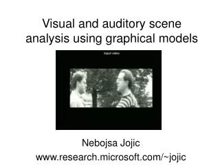
Visual and auditory scene analysis using graphical models
Visual and auditory scene analysis using graphical models. Nebojsa Jojic www.research.microsoft.com/~jojic. People. Interns: Anitha Kannan Nemanja Petrovic Matt Beal. Collaborators: Brendan Frey Hagai Attias Sumit Basu. Windows: Ollivier Colle Nenad Stefanovic Sheldon Fisher.

Visual and auditory scene analysis using graphical models
E N D
Presentation Transcript
Visual and auditory scene analysis using graphical models Nebojsa Jojic www.research.microsoft.com/~jojic
People Interns: Anitha Kannan Nemanja Petrovic Matt Beal Collaborators: Brendan Frey Hagai Attias Sumit Basu Windows: Ollivier Colle Nenad Stefanovic Sheldon Fisher Soon to join: Trausti Kristijansson
Our representation • Objects rather than pixels • regions with stable appearance over time • moving coherently • occluding each other • subject to lighting changes • associated audio and its structure • Applications: compression, editing, watermarking, indexing, search/retrieval, …
A structured probability model • Reflects desired structure • Randomly generates plausible images • Represents the data by parameters
Recognition Tracking Feature extraction Contrast enhancement Intrinsic appearance Intrinsic appearance Illumination Illumination Mask Mask Appearance Appearance Position Position Observed image Observed image (a) Block processing (b) Structured probability model
Inference, learning and generation • Inference (inverting the generative process) • Bayesian inference • Variational inference • Loopy belief propagation • Sampling techniques • Learning • Expectation maximization (EM) • Generalized EM • Variational EM • Generation • Editing by changing some variables • Video/audio textures
Basic flexible layer model s1 m1 s2 m2 T1 T2 T1s1 T1m1 T2s2 T2m2 x
Multiple flexible layers … Layer 1 variables Layer L variables Class c1 Class cL Appearance Mask s1 m1 sL mL T1 TL … Transformation T1s1 T1m1 TLsL TLmL x Observed image
Probability distribution c=1 c=2 c=3
T1s1 T1m1 TLsL TLmL x Layer equation (Adelson et al) …
= + • •( + • ) •
Likelihood, learning, inference • Pdf of x, p(x) = integral over the product of all the conditional pdfs • Inference: hard! • Maximizing p({xt}) efficiently done using variational EM: • Infer hidden variables • Optimize parameters keeping the above fixed • Loop
Video indexing:Six break points vs. six things in video • Traditional video segmentation: Find breakpoints Example: MovieMaker (cut and paste) • Our goal: Find possibly recurring scenes or objects timeline 1 2 3 2 4 1 4 3 2 3 2 3 5 6
Video clustering Class index Class mean (representative image) Shift Mean with added variability Transformed (shifted image) Transformed image with added non-uniform noise Optimizing average or minimum frame likelihood
Video indexing:Six break points vs. six things in video • Traditional video segmentation: Find breakpoints Example: MovieMaker (cut and paste) • Our goal: Find possibly recurring scenes or objects timeline 1 2 3 2 4 1 4 3 2 3 2 3 5 6
Video indexing:Six break points vs. six things in video Differences: timeline • A class is detected at multiple intervals on the timeline. For example, class 1 models a baby’s face. Break pointers miss it at the second occurrence. The class occurs more in the rest of the sequence 1 2 3 2 4 1 4 3 2 3 2 3 5 6
Video indexing:Six break points vs. six things in video Differences: timeline One long shot contains a pan of the camera back and forth among three scenes (classes 2,3 and 5) 1 2 3 2 4 1 4 3 2 3 2 3 5 6
Video indexing:Six break points vs. six things in video Differences timeline Two shots detected just because the camera was turned off and then on with a slightly different vantage point are considered a single scene class. 1 2 3 2 4 1 4 3 2 3 2 3 5 6
Adding other variables (see also www.research.microsoft.com/users/jojic/FlexibleSprites.htm) • Subspace variables (for PCA-like models) • Deformation fields • Cluster variables • Illumination • Texture • Time series model • Context • Rendering model
Adding other modalities and/or sensors Intrinsic appearance Intrinsic appearance Illumination Illumination Mask Mask Appearance Appearance Position Position audio model time delay A Mic 1 Mic 2 Observed image Observed audio
Challenges • Computational complexity • Achieving modularity in inference • Generality at expense of optimality?
Rewards Object-based media • Meta data, annotations • Automated search • Compression • Manipulability Structured probability models • Ease of development • Unified framework • Compatible with other reasoning engines
A unified theory of natural signals • Probabilistic formulation: • flexibility in “stability” and “coherence” • unsupervised learning possible • Structured probability models: • Random variables: observed and hidden • Dependence models • Inference and learning engines
h Variational inference and learning Gaussian Multinomial • Generalized E step (variational inference): optimize Bn wrt q(hn), keeping the model fixed • 2. Generalized M step: optimize Bn wrt to model parameters, keeping q(hn) fixed
h Use of FFTs in inference Gaussian Multinomial Optimizing terms of the form q(T) (x-Ts)T(x-Ts) requires xTTs for all T – correlation if T are shifts! In FFT domain: X*S
h Use of FFTs in learning Gaussian Multinomial Computing expectations of the form q(T)TTx reduces to QX in FFT domain!
Media is “multidisciplinary” • Image processing • Filtering, compression, fingerprinting, hashing, scene cut detection • Telecommunications • Encryption, transmission, error correction • Computer vision • Motion estimation, structure from motion, motion/object recognition, feature extraction • Computer graphics • Rendering, mixing natural and synthetic, art • Signal processing • Speech recognition, speaker detection/tracking, source separation, audio encoding, fingerprinting
Lack of a new unifying theory • The old general theory of signal decomposition lacked: • Semantics in the representation (objects, motion patterns, illumination conditions, …) • Notion of unknown and hidden cases • Narrow application-dependent frameworks: • Structure from motion • Video segmentation and indexing • Face recognition • HMMs for speech recognition • …