Download
1 / 33
330 likes | 442 Vues
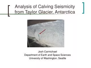
Analysis of Calving Seismicity from Taylor Glacier, Antarctica. Josh Carmichael Department of Earth and Space Sciences University of Washington, Seattle. What I will tell You. Part I: Introduction to the science Calving: what it is, why you should care

E N D
Analysis of Calving Seismicity from Taylor Glacier, Antarctica Josh Carmichael Department of Earth and Space Sciences University of Washington, Seattle
What I will tell You Part I: Introduction to the science • Calving: what it is, why you should care • Seismology: what it is, some theory, applied to glaciology • Problem Statement: how to identify a calving event from a few seismometers • The Seismogram: part path, part calving source • Calving source as a dislocation on a fault • Expressed features along the path from a source to a receiver
What I will tell You (cont…) Part II: Analysis of Seismograms • Interlude: Questions so far? • Cross Correlation of waveforms, what it is, what it might say • Polarization analysis: direction energy comes from • Fourier Transforms of time series, power spectra, interpretation • Other ideas
Calving of Dry Land Glaciers • Calving: The partial or full collapse of an ice shelf—usually from free surface evolution • Illustration: why read this slide when you can watch the movie • What you just saw: • 10 days of visible buckling + deformation, prior to calving • Complete calving > 3 m thick ice column ~35 meters long in < 1 day
Why Study Calving? (Who Cares?) • Climatologists, Glaciologists: use Antarctica and Greenland to study climate change • Calving is the dominant mechanism for ice loss in Antarctica • Most models don’t assume the existence of ice cliffs, let alone, calving bad • Need way to measure calving frequency!
Why Seismology can Help: Calving Ground Displacement • Calving events shake ice and ground E,N,Z recorded by seismograms • Sensor sample rate = 200Hz • Instrumental temperature resilience: operates to -40 • IF calving seismicity is unambiguous can count events • Can estimate calving locations (inverse problem)
The Array 1000 meters
A Model for Calving Source Decomposition • Pre-Calve: Column loads glacier; deformation time scale ~10 days; damage evolution to crack formation • Precursor events seismically similar
A Model for Calving Source Decomposition • Crack propagation along damaged-weakened regions • Column unloads free surface
A Model for Calving Source Decomposition • Energy scattering from column collapse; incoherent, high frequency Energy Scatter
Problem Statement • Can a calving event be unambiguously identified in the seismic record? • Can it tell us about seasonal precursor events? Bottom-Up Problem: Seasonal calving statistics realizable givencalving waveforms can be recognized
Some Basic Questions Concerning the Problem: • What else excites the sensor? • Even if you know ice calved, is it distinct on the seismogram? (source uniqueness?) • The opposing question: Will separate calving events look similiar? (well-posed?) • What does calving look like? (characterization) The big question We will come back to this
Enter Non-Global Seismology • Experimental Seismology: using ground motion records to infer structure, or nature of source • Detectable by seismometers: helicopters, tides, landslides, lightening, anything that is loud… • “Seismograms”: ground motion waveforms (velocity usually what is really recorded). • Differences from global seismology: less attenuation, rays sample local structure only, shorter wavelengths, tighter array coverage.
Seismic Waves in Boring Media S • Equation of motion x S V Impulsive force* Green’s function* mpq= From Betti’s Rep. Thm. for an internal dislocation on S * If you care: ask me what a delta function really is, or what LG = d means rigorously, after this talk
What Displacement Solutions Look Like • For an infinite, homogeneous, uniform medium, with no initial motion and a point dislocation: • For half-space, with traction-free boundary conditions, with no initial motion or body forces:
The Displacement Field Integral Units of moment per unit area Time shift convolution Couple magnitude Integrand is inner product of 2nd and 3rd order tensor: result is vector xq • The displacement field representation is a convolution of two tensors—a smoothing operation • The Green’s function spatial derivative is physically a force couple, with moment arm in the xqdirection xp
Seismic Waves in Boring Media (continued) • The point: displacement on S determines displacement everywhere thru a convolution of the impulse response’s derivative with the slip function • Interpretation: Equivalent to a sum of force couples distributed over internal surface: x3 CLVD Moment Density Tensor
Examples of Moment Tensor Physical Realizations • Respectively, left to right: (1) An explosion or implosion (2) The compensated linear vector dipole (3) mode III failure (4) mode II failure
What’s Seen by the Sensor • A seismogram is a convolution of the slip contribution and the source: W(t) Green function = source Slip, material effects • Convolution theorem turns integration into multiplication, but freq. domain loses phase info.
What to Expect Beneath the Glacier and Sand ~50m ~30m ~200m-500m • Sensors close to source see top layer effects • If we ignore deeper layering, must ignore arrivals corresponding to smaller ray parameters
Summary So Far Seismogram for an internal dislocation in the ice: • Same location events may differ only in source • Same source events may differ only in their path • Identical calving events at distinct locations have identical waveforms, minus the path • Frequency domain turns temporal convolution into multiplication
Now For Some Data Ideas on how to Analyze the Data
Time, Location of a Calving Event • Broken tilt sensors and cables time of calving • GPS locations known • Search through record ~10 days prior to total data loss
Plan: Find Similar Waveforms from Same Location • From previous slides, we expect waveforms for similar events to match; • We know from observation where the most actively calving region is • First off: we find events that arrive @ the cliff-adjacent stations first and compare…(no location necessary)
Cross-Correlation: Test for Waveform Similarity • Global maxima of a the cross-correlated function value of t gives max. overlap • High correlation coefficient high waveform similarity
Structure Features or Source? Closer station: rich in high freq. Distant station: rich in lower freq. Same Event Common Spectral Amplitude Most similar to calving event • Spectral peaks obvious on each station • Glacial spatial features, wave speed standing waves trapped in ice could have 23Hz peak
Application of Cross Correlation: Categorizing Waveforms Vertical Component R > 0.97 Antarctic Day Antarctic Day • Is this all thermal skin cracking? • Is any of this actually calving? Log[ vL2/vH2 ] vs. time
Organizing Multiplets • Multiplet: several events originating from the same location, separated temporally • Polarization: The direction of particle motion for a wave; seismic waves characterized by 3 polarization vectors
Polarization Analysis of Multiplets • Construct a matrix of displacement in each direction • Form a 3x3 matrix • Perform an eigenvalue decomposition (SVD also permissible) • The magnitude of the eigenvalue ratio: provides a measure of size of polarization axes
Polarization Data rotated Eigenvalue Ratios Largest Eigenvectors
Future Directions (if any) • Model the calving of large ice columns near failure time (“easy part”) • Pre-Cursory event modeling of unstable cliff face (“hard part”) • Hard part involves multiple time scales: • Ice wall deformation (~50 days) • Crevasse opening (~10 days) • Fault plane growth, generation (~ 1 hour?) • Rupture (~ 1 sec)
Summary • Calving is the most prominent form of ice loss from Antarctica • Sensors: see u = convolution of couple distribution over plane w/moment density and path • Data shows: • Diurnal fluctuations in warm months of seismic activity • Waveforms may be categorized into “similarity” sets for discerning source differences • Polarization shows activity swarms from same direction
Thanks To... • Ken Creager • Erin Pettit • Matt Szundy • Matt Hoffman • Erin Whorton • AMATH