Lecture 8 Tracers for Gas Exchange
Lecture 8 Tracers for Gas Exchange. Examples for calibration of gas exchange using: 222 Rn – short term 14 C - long term. E&H Sections 5.2 and 10.2. Rates of Gas Exchange Stagnant Boundary Layer Model. well mixed atmosphere. C g = K H P gas = equil. with atm. ATM. 0. OCN.

Lecture 8 Tracers for Gas Exchange
E N D
Presentation Transcript
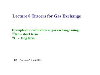
Lecture 8 Tracers for Gas Exchange Examples for calibration of gas exchange using: 222Rn – short term 14C - long term E&H Sections 5.2 and 10.2
Rates of Gas Exchange Stagnant Boundary Layer Model. well mixed atmosphere Cg = KH Pgas = equil. with atm ATM 0 OCN Stagnant Boundary Layer – transport by molecular diffusion ZFilm Depth (Z) CSW well mixed surface SW Z is positive downward C/ Z = F = + (flux into ocean) see: Liss and Slater (1974) Nature, 247, p181 Broecker and Peng (1974) Tellus, 26, p21 Liss (1973) Deep-Sea Research, 20, p221
Expression of Air -Sea CO2 Flux Need to calibrate! S – Solubility From Temperature & Salinity k = piston velocity = D/Zfilm From wind speed F = k s (pCO2w- pCO2a) = K ∆ pCO2 pCO2a pCO2w From measurements at sea From CMDL CCGG network
Gas Exchange and Environmental Forcing: Wind Wanninkhof, 1992 from 14C Liss and Merlivat,1986 from wind tunnel exp. ~ 5 m d-1 Example conversion: 20 cm hr-1 = 20 x 24 / 102 = 4.8 m d-1
Analytical Method for 222Rn and 226Ra Analyze for 222Rn immediately, then 226Ra later (after 20 days) 5 half-lives charcoal liquid N2 222Rn Activity is what is measured. Not concentration! SW 226Ra Apply the principle of secular equilibrium!
226Ra profiles in Atlantic and Pacific Q. What controls the ocean distributions of 226Ra?
226Ra – Si correlation – Pacific Data Q. Why is there a hook at the end? You can calculate 226Ra from Si!
226Ra source from the sediments Edmond et al (1979) JGR 84, 7809-7826
222Rn Example Profile from North Atlantic Does Secular Equilibrium Apply? t1/2222Rn << t1/2 226Ra (3.8 d) (1600 yrs) YES! Then.. A226Ra = A222Rn 222Rn 226Ra Why is 222Rn activity less than 226Ra?
222Rn is a gas and the 222Rn concentration in the atmosphere is much less than in the ocean mixed layer (Zmlmixed layer). Thus, there is a net evasion (gas flux) of 222Rn out of the ocean. The simple 1-D 222Rn balance for the mixed layer, with thickness Zml, ignoring horizontal advection and vertical exchange with deeper water, is: d222Rn/dt = sources – sinks = decay of 226Ra – decay of 222Rn - gas exchange to atmosphere Zmll222Rnd[222Rn]/dt = Zmll226Ra [226Ra] – Zmll222Rn [222RnML] - D/Zfilm{ [222Rnatm] – [222RnML]} Knowns: l222Rn, l226Ra, DRn Measure: Zml,A226Ra, A222Rn, d[222Rn]/dt Solve for Zfilm
Zmlλ222Rnd[222Rn]/dt = Zmlλ226Ra[226Ra] – Zmlλ222Rn[222Rn] - D/Zfilm { [222Rnatm] – [222RnML]} ZmlδA222Rn/ δt = Zml(A226Ra – A222Rn) + D/Z (CRn, atm – CRn,ML) Note: diffusion is expressed in terms of concentrations not activities atm Rn = 0 for SS = 0 Then -D/Z ( – CRn,ml) = Zml(A226Ra – A222Rn) +D/Z (ARn,ml/λRn) = Zml(A226Ra – A222Rn) +D/Z (ARn,ml) =ZmlλRn(A226Ra – A222Rn) ZFILM = D (A222Rn,ml) / ZmlλRn(A226Ra – A222Rn) ZFILM = (D /ZmlλRn) ()
Stagnant Boundary Layer Film Thickness Z = DRn / Zfilm l222Rn (1/A226Ra/A222Rn) ) - 1 Histogram showing results of film thickness calculations from many stations. Organized by ocean and by latitude Average Zfilm = 28 mm • Q. What are limitations of • this approach? • unrealistic physical model • steady state assumption • short time scale
Cosmic Ray Produced Tracers – including 14C Cosmic ray interactions produce a wide range of nuclides in terrestrial matter, particularly in the atmosphere, and in extraterrestrial material accreted by the earth. IsotopeHalf-lifeGlobal inventory (pre-nuclear) 3H 12.3 yr 3.5 kg 14C 5730 yr 54 ton 10Be 1.4 x 10⁶yr 430 ton 7Be 54 d 32 g 26Al 7.4 x 10⁵yr 1.7 ton 32Si 276 yr 1.4 kg
Carbon-14 is produced in the upper atmosphere as follows: Cosmic Ray Flux Fast Neutrons Slow Neutrons + 14N* 14C (protons)(thermal) (5730 yrs) From galactic cosmic rays from supernova, which are more energetic than solar wind. So these are not from the sun. The overall reaction is written: 14N + n 14C + p (7n, 7p) (8n, 6p) So the production rate from cosmic rays can be calculated For more detail see: von Blanckenburg and Willenbring (2014) Elements, 10, 341-346
Bomb Fallout Produced Tracers Nuclear weapons testing and nuclear reactors (e.g. Chernobyl) have been an extremely important sources of nuclides used as ocean tracers. The main bomb produced isotopes have been: IsotopeHalf LifeDecay 3H 12.3 yrs beta 14C 5730 yrs beta 90Sr 28 yrs beta 238Pu 86 yrs alpha 239+240Pu 2.44 x 10⁴yrs alpha 6.6 x 10³yrs alpha 137Cs 30 yrs beta, gamma Nuclear weapons testing has been the overwhelmingly predominant source of 3H, 14C, 90Sr and 137Cs to the ocean. Nuclear weapons testing peaked in 1961-1962. Fallout nuclides act as "dyes" Another group of man-made tracers that fall in this category but are not bomb-produced and are not radioactive are the chlorofluorocarbons (CFCs).
Atmospheric 14CO2 in the second half of the 20th century. The figure shows the 14C / 12C ratio relative to the natural level in the atmospheric CO2 as a function of time in the second half of the 20th century.
The bomb spike: surface ocean and atmospheric Δ14C since 1950 • Massive production in nuclear tests ca. 1960 (“bomb 14C”) • Through air-sea gas exchange, the ocean took up ~half of the bomb 14C by the 1980s data: Levin & Kromer 2004; Manning et al 1990; Druffel 1987; Druffel 1989; Druffel & Griffin 1995 bomb spike in 1963
Comparison of 14C in surface ocean Pre-nuclear (1950s) and nuclear (1970s) Atlantic Indian Pacific
Example – Use 14C to calculate ZFILM using the Stagnant Boundary Layer 14Catm Use Pre-bomb 14C – assume steady state 1-box model source = sink 14C from gas exchange = 14C lost by decay [14C] 14C decay Assume [CO2]top = [CO2]bottom = [CO2]surface ocean (e.g. no CO2 gradient, only a 14C gradient)
Assume D = 3 x 10⁻² m2 y-1 h = 3800m l-1 = 8200 y [CO2]surf = 0.01 moles m-3 [DIC]ocean = 2.4 moles m-3 a14CO2/aCO2 = 1.015 (14C-CO2 is more soluble than CO2)(a equals solubility constant) (14C/C) surf = 0.96 (14C/C)atm (14C/C)deep = 0.84 (14C/C)atm Then: Zfilm = 1.7 x 10⁻⁵ m = 17 mm
Example – 14C Deep Ocean Residence Time substitute for B vmix in cm yr-1; vC in cm yr-1 x mol cm-3
Rearrange and Solve for Vmix Use pre-nuclear 14C data when surface 14C > deep 14C (14C/C)deep = 0.81 (14C/C)surf Vmix = (200 cm y-1) A A = ocean area for h = 3200m thus age of deep ocean box (t) t = 3200m / 2 my-1 = 1600 years
Example: What is the direction and flux of oxygen across the air-sea interface given? PO2 = 0.20 atm KH,O2 = 1.03 x 10⁻³ mol kg-1 atm-1 O2 in mixed layer = 250 x 10-6 mol l-1 (assume 1L = 1 kg) The wind speed (U10) = 10 m s-1 Answer: O2 in seawater at the top of the stagnant boundary layer = KH PO2 = 1.03 x 10-3 x 0.20 = 206 x 10-6 mol l-1 So O2ml > O2atm and the flux is out of the ocean. What is the flux? With a wind speed = 10 m s-1, the piston velocity (k) = 5 m d-1 DC = (250 – 206) x 10-6 = 44 x 10-5 mol l-1 Flux = 5 m d-1 x 44 x 10-6 mol l-1 x 10³ l m-3 = 5 x 44 x 10-6 x 103 = 220 x 10-3 mol m-2 d-1
Example The activity of 222Rn is less than that of 226Ra in the surface water of the North Atlantic at TTO Station 24 (western North Atlantic). Calculate the thickness of the stagnant boundary layer (ZFILM). A226Ra = 8.7 dpm100 L-1 A222Rn = 6.9 dpm100 L-1 Assume: λ222Rn= 2.1 x 10⁻⁶ s-1 D222Rn = 1.4 x 10⁻⁹ m2 s-1 Zml= 40m Answer: ZFILM = 40 x 10-6 m
Tritium(3H) is produced from cosmic ray interactions with N and O. After production it exists as tritiated water ( H - O -3H ), thus it is an ideal tracer for water. Tritium concentrations are TU (tritium units) where 1 TU = 1018 (3H / H) Thus tritium has a well defined atmospheric input via rain and H2O vapor exchange. Its residence time in the atmosphere is on the order of months. In the pre-nuclear period the global inventory was only 3.5 kg which means there was very little 3H in the ocean at that time. The inventory increased by 200x and was at a maximum in the mid-1970s
Tritium (3H) in rain and surface SW
Tritium is a conservative tracer for water (as HTO) – thermocline penetration Eq Meridional Section in the Pacific
Atmospheric Record of Thermocline Ventilation Tracers Conservative, non-radioactive tracers (CFC-11, CFC-12, CFC13, SF6) Time series of northern hemisphere atmospheric concentrations and tritium in North Atlantic surface waters
226Ra Distributions Example 226Ra Profile South Atlantic at 15°S ; 29.5°W
222Rn as a tracer for gas exchange d222Rn/dt = sources – sinks = decay of 226Ra – decay of 222Rn - gas exchange to atmosphere