Solving Op Amp Stability Issues
Solving Op Amp Stability Issues. (For Voltage Feedback Op Amps) Tim Green & Collin Wells Precision Analog Linear Applications. www.ti.com/techdaytoolscoupon. Check your Tech Day bags!. #TItechday . TI Precision Designs Three design levels from the desks of our analog experts.

Solving Op Amp Stability Issues
E N D
Presentation Transcript
Solving Op Amp Stability Issues (For Voltage Feedback Op Amps) Tim Green & Collin Wells Precision Analog Linear Applications
www.ti.com/techdaytoolscoupon Check your Tech Day bags! #TItechday
TI Precision Designs Three design levels from the desks of our analog experts. TI Precision Designs Hub blog Get tips, tricks and techniques from TI precision analog experts Get to both at: http://www.ti.com/ww/en/analog/precision-designs/ #TItechday
Overview • Main Presentation Focus: • Op Amp Stability Basics • Stability Analysis – Method 1 : Loaded Aol & 1/b Technique • A) Riso Compensation Technique for Output Capacitive Loads • Stability Analysis – Method 2 : Aol & 1/b Technique • CF Compensation Technique for Input Capacitance • Stability Tricks and Rules of Thumb • Appendix: • Additional Useful Tools for your Analog Stability Toolbox • Op Amp Output Impedance • Pole and Zero: Magnitude and Phase on Bode Plots • Dual Feedback Paths and 1/b • Non-Loop Stability Problems • 2) Nine different ways to stabilize op amps with capacitive loads • A) Definition by example using TINA-TI simulations
The Culprits Output Capacitive Loads! Cable/Shield Drive! MOSFET Gate Drive! Reference Buffers! Input Capacitance and Large Value Resistors Large Value Resistors or Low-Power Circuits! Transient Suppression! Transimpedance Amplifiers!
Just Plain Trouble! Inverting Input Filter?? Oscillator Output Filter?? Oscillator
But it worked fine in the lab! Transient on: +Input or –Input Vcc or Vee Output But I’m only using it at DC! Check ALL Op Amp Circuits for Stability regardless of their closed loop signal frequency of operation!
Recognize Amplifier Stability Issues on the Bench • Required Tools: • Oscilloscope • Signal Generator • Other Useful Tools: • Gain / Phase Analyzer • Network / Spectrum Analyzer
Recognize Amplifier Stability Issues • Oscilloscope - Transient Domain Analysis: • Oscillations or Ringing • Overshoots • Unstable DC Voltages • High Distortion
Recognize Amplifier Stability Issues • Gain / Phase Analyzer - Frequency Domain: - Peaking, Unexpected Gains, Rapid Phase Shifts
Poles and Bode Plots • Pole Location = fP • Magnitude = -20dB/Decade Slope • Slope begins at fP and continues down as frequency increases • Actual Function = -3dB down @ fP • Phase= -45°/Decade Slope through fP • Decade Above fP Phase = -90° (-84.3°) • Decade Below fP Phase = 0° (-5.7°)
Zeros and Bode Plots • Zero Location = fZ • Magnitude = +20dB/Decade Slope • Slope begins at fZ and continues up as frequency increases • Actual Function = +3dB up @ fZ • Phase = +45°/Decade Slope through fZ • Decade Above fZ Phase = +90° (+84.3°) • Decade Below fZ Phase = 0° (5.7°)
Capacitor and Inductor - Impedance vs Frequency Low frequency= High Impedance High frequency= High Impedance Low frequency= Low Impedance High frequency= Low Impedance
Op-Amp Loop Gain Model VOUT/VIN = Acl = Aol/(1+Aolβ) If Aol >> 1 then Acl ≈ 1/β Aol: Open Loop Gain β: Feedback Factor Acl: Closed Loop Gain
b and 1/b • β is easy to calculate as feedback network around the Op Amp • 1/β is reciprocal of β • Easy Rules-Of-Thumb and Tricks to Plot 1/β on Op Amp Aol Curve • Plotting Aol Curve and 1/β Curve shows Loop Gain
Amplifier Stability Criteria VOUT/VIN = Aol / (1+ Aolβ) If: Aolβ = -1 Then: VOUT/VIN = Aol / 0 ∞ If VOUT/VIN = ∞ Unbounded Gain Any small changes in VIN will result in large changes in VOUT which will feed back to VIN and result in even larger changes in VOUT OSCILLATIONS INSTABILITY !! Aolβ: Loop Gain Aolβ = -1 Phase shift of +180°, Magnitude of 1 (0dB) fcl: frequency where Aolβ = 1 (0dB) Stability Criteria: At fcl, where Aolβ = 1 (0dB), Phase Shift < +180° Desired Phase Margin (distance from +180° Phase Shift) > 45°
Traditional Loop Gain Test Op Amp Loop Gain Model Op Amp is “Closed Loop” Loop Gain Test: (An Open Loop Test) Break the Closed Loop at b Ground VIN Inject AC Source, VTest, into b Aolβ = VOUT
Traditional Loop Gain Test Op Amp Loop Gain Model Op Amp is “Closed Loop” VOUT/VIN = Aol / (1+Aolb) SPICE Loop Gain Test: Op Amp Loop Gain Test is an “Open Loop” Test SPICE finds a DC Operating Point before it does an AC Analysis so loop must be closed for DC and open for AC. Break the Closed Loop at VOUT Ground VIN source impedance low for AC analysis Inject: AC Source, VTest, into RF (Inject: AC Source into High Impedance Node) Read: Aolβ = Loop Gain = VOUT (Read: Loop Gain from Low Impedance Node)
SPICE Loop Gain Test DC Analysis DC Analysis DC Analysis DC Equivalent Circuit AC Equivalent Circuit
Loop Gain (Aolb) from Aol and 1/b Plot (dB) 1/β on Op Amp Aol (dB) Aolβ = Aol(dB) – 1/β(dB) Aolβ = Aol / (1/β) = Aolβ Note how Aolβ changes with frequency
“Rate-of-Closure” Stability Criteria using 1/β & Aol At fcl: Loop Gain (Aolb) = 1 (0dB) Rate-of-Closure @ fcl = (Aol slope – 1/β slope) *20dB/decade Rate-of-Closure @ fcl = STABLE **40dB/decade Rate-of-Closure @ fcl = UNSTABLE
Loop Gain (Aolb) Example Rate-of-Closure @ fcl = 40dB/decade UNSTABLE! Example 1: Note locations of poles and zeros in Aol & 1/b
Loop Gain (Aolβ) Plotfrom Aol & 1/β Plot Loop Gain (Aolb) Phase at fcl: Phase Shift = -180 Phase Margin = 0 To Plot Aolβ from Aol & 1/β Plot: Poles in Aol curve are Polesin Aolβ (Loop Gain)Plot Zeros in Aol curve areZeros in Aolβ (Loop Gain) Plot Poles in 1/β curve areZeros in Aolβ (Loop Gain) Plot Zeros in 1/β curve are Polesin Aolβ ( Loop Gain) Plot [Remember: β is the reciprocal of 1/β] Example 1: Note locations of poles and zeros in Loop Gain
1/β Always = Closed Loop Response VOUT/VIN = Aol/(1+Aolβ) At fcl: Aolβ = 1 VOUT/VIN = Aol/(1+1) ~ Aol No Loop Gain left to correct for errors VOUT/VIN follows the Aol curve at f > fcl Note: 1/β is the AC, Small Signal, Closed Loop, ”Noise Gain” for the Op Amp. VOUT/VIN is often NOT the same as 1/β.
1/β “First Order Analysis” for ZF • 1/βLow Frequency = RF/RI = 100 40dB Cp = Open at Low Frequency • 1/βHigh Frequency = (Rp//RF)/RI ≈ Rp/RI = 10 20dB Cp = Short at High Frequency • Pole in 1/β when Magnitude of XCp = RF Magnitude XCp = 1/(2∙п∙f∙Cp) fp = 1/(2∙п∙RF∙Cp) = 1kHz • Zero in 1/β when Magnitude of XCp = Rp fz = 1/(2∙п∙Rp∙Cp) = 10kHz
TINA SPICE: 1/β for ZF Lo f Hi f
1/β“First Order Analysis” for ZI • 1/βLow Frequency = RF/RI = 10 20dB Cn = Open at Low Frequency • 1/βHigh Frequency = RF/(RI//Rn) ≈ RF/Rn =100 40dB Cn = Short at High Frequency • Zero in 1/β when Magnitude of XCn = RI Magnitude XCn = 1/(2∙п∙f∙Cn) fz = 1/(2∙п∙RI∙Cn) = 1kHz • Pole in 1/β when Magnitude of XCn = Rn fp = 1/(2∙п∙Rn∙Cn) = 10kHz
TINA SPICE: 1/β for ZI Hi f Lo f
Stability Analysis - Method 1 (Loaded Aol & 1/b Technique)(Riso Compensation)
Capacitive Loading on Op Amp Outputs Unity Gain Buffer Circuits Circuits with Gain Will this circuit behavior get you a raise in pay?
Loaded Aol Model fp2
Loaded Aol Model fp2 Aol fp1 Aol Load + fp1 Loaded Aol fp2 = Note: Addition on Bode Plots = Linear Multiplication
Loaded Aol – Loop Gain & Phase Phase Margin at fcl
Riso Compensation Riso will add a zero in the Loaded Aol Curve
Riso Compensation Theory fp2 fz1
Riso Compensation Theory fp1 Aol fp2 fz1 Aol Load + fp1 Loaded Aol fz1 fp2 = Note: Addition on Bode Plots = Linear Multiplication
Riso Compensation Design Steps • Determine fp2 in Loaded Aol due to CLoad • Measure in SPICE with CLoad on Op Amp Output • Plot fp2 on original Aol to create new Loaded Aol • 3) Add Desired fz2 on to Loaded Aol Plot for Riso Compensation • Keep fz1 < 10*fp2 (Case A) • Or keep the Loaded Aol Magnitude at fz1 > 0dB (Case B) • (fz1>10dB will allow for Aol variation of ½ Decade in Unity Gain Bandwidth) • 4) Compute value for Riso based on plotted fz1 • 5) SPICE simulation with Riso for Loop Gain (Aolb) Magnitude and Phase • Adjust Riso Compensation if greater Loop Gain (Aolb) phase margin desired • Check closed loop AC response for VOUT/VIN • Look for peaking which indicates marginal stability • Check if closed AC response is acceptable for end application • Check Transient response for VOUT/VIN • Overshoot and ringing in the time domain indicates marginal stability • Determine if settling time is acceptable for end application
1),2) Loaded Aol and fp2 Case A, CLoad=1uF, fp2=2.98kHz Case B, CLoad=2.9nF, fp2=983.37kHz
3) Add fz1 on Loaded Aol Case A, CLoad=1uF, fz1=29.8kHz Case B, CLoad=2.9nF, fz1=4.07MHz
4) Compute Value for Riso Case A, CLoad=1uF, fz1=29.8kHz Case B, CLoad=2.9nF, fz1=4.07MHz
5),6) Loop Gain, Case A Phase Margin at fcl = 87.5 degrees