Summary of Papers

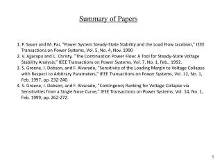
1. Summary of Papers 1. P. Sauer and M. Pai, “Power System Steady-State Stability and the Load Flow Jacobian,” IEEE Transactions on Power Systems, Vol. 5, No. 4, Nov. 1990 2. V. Ajjarapu and C. Christy, “The Continuation Power Flow: A Tool for Steady-State Voltage Stability Analysis,” IEEE Transactions on Power Systems, Vol. 7, No. 1, Feb., 1992. 3. S. Greene, I. Dobson, and F. Alvarado, “Sensitivity of the Loading Margin to Voltage Collapse with Respect to Arbitrary Parameters,” IEEE Transactions on Power Systems, Vol. 12, No. 1, Feb. 1997, pp. 232-240. 4. S. Greene, I. Dobson, and F. Alvarado, “Contingency Ranking for Voltage Collapse via Sensitivities from a Single Nose Curve,” IEEE Transactions on Power Systems, Vol. 14, No. 1, Feb. 1999, pp. 262-272.

2. Voltage Security • Voltage security is the ability of the system to maintain • adequate and controllable voltage levels at all system load buses. • The main concern is that voltage levels outside of a specified • range can affect the operation of the customer’s loads. • Voltage security may be divided into two main problems: • 1. Low voltage: voltage level is outside of pre-defined range. • 2. Voltage instability: an uncontrolled voltage decline. • You should know that • low voltage does not necessarily imply voltage instability • no low voltage does not necessarily imply voltage stability • voltage instability does necessarily imply low voltage

3. Resources • There have been several individuals that have significantly • progressed the field of voltage security. These include: • Ajjarapu from ISU • Van Cutsem: See the book by Van Cutsem and Vournas. • Alvarado, Dobson, Canizares, & Greene: • There are a couple other texts that provide good treatments of • the subject: • Carson Taylor: “Power System Voltage Stability” • Prabha Kundur: “Power System Stability & Control”

4. Our treatment of voltage security will proceed as follows: • Voltage instability in a simple system • Voltage instability in a large system • Brief treatment of bifurcation analysis • Continuation power flow (path following) methods • Sensitivity methods

5. Voltage instability in a simple system Consider the per-phase equivalent of a very simple three phase power system given below: V1 V2 Z=R+jX Node 1 Node 2 I + + V2 V1 _ _ S12 SD=-S12

6. Note B>0 Let G=0. Then….

7. Now we can get SD=PD+jQD=-(P21+jQ21) by • - exchanging the 1 and 2 subscripts in the previous equations. • - negating Define 12 =1- 2

8. Define:  is the power factor angle of the load, i.e., Then we can also express SD as: Note that phi, and therefore beta, is positive for lagging, negative for leading. Define β=tan. Then

9. So we have developed the following equations…. Equating the expressions for PD and for QD, we have: Square both equations and add them to get…..

10. Manipulation yields: Note that this is a quadratic in |V2|2. As such, it has the solution:

11. Let’s assume that the sending end voltage is |V1|=1.0 pu and B=2 pu. Then our previous equation becomes: % pf = 0.97 lagging beta=0.25 pdn=[0 0.1 0.2 0.3 0.4 0.5 0.6 0.7 0.78]; v2n=sqrt((1-beta.*pdn - sqrt(1-pdn.*(pdn+2*beta)))/2); pdp=[0.78 0.7 0.6 0.5 0.4 0.3 0.2 0.1 0]; v2p=sqrt((1-beta.*pdp + sqrt(1-pdp.*(pdp+2*beta)))/2); pd1=[pdn pdp]; v21=[v2n v2p]; % pf = 1.0 beta=0 pdn=[0 0.1 0.2 0.3 0.4 0.5 0.6 0.7 0.8 0.9 0.99]; v2n=sqrt((1-beta.*pdn - sqrt(1-pdn.*(pdn+2*beta)))/2); pdp=[0.99 0.9 0.7 0.6 0.5 0.4 0.3 0.2 0.1 0]; v2p=sqrt((1-beta.*pdp + sqrt(1-pdp.*(pdp+2*beta)))/2); pd2=[pdn pdp]; v22=[v2n v2p]; % pf = .97 leading beta=-0.25 pdn=[0 0.1 0.2 0.3 0.4 0.5 0.6 0.7 0.8 0.9 1.0 1.1 1.2 1.3]; v2n=sqrt((1-beta.*pdn - sqrt(1-pdn.*(pdn+2*beta)))/2); pdp=[1.3 1.2 1.1 1.0 0.9 0.7 0.6 0.5 0.4 0.3 0.2 0.1 0]; v2p=sqrt((1-beta.*pdp + sqrt(1-pdp.*(pdp+2*beta)))/2); pd3=[pdn pdp]; v23=[v2n v2p]; plot(pd1,v21,pd2,v22,pd3,v23) You can make the P-V plot using the following matlab code.

12. Plots of the previous equation for different power factors |V2| Real power loading, PD

13. Some comments regarding the PV curves: • 1. Each curve has a maximum load. This value is typically called the maximum system load or the system loadability. • 2. If the load is increased beyond the loadability, the voltages will • decline uncontrollably. • 3. For a value of load below the loadability, there are two • voltage solutions. The upper one corresponds to one that can be • reached in practice. The lower one is correct mathematically, but I • do not know of a way to reach these points in practice. • 4. In the lagging or unity power factor condition, it is clear that the • voltage decreases as the load power increases until the loadability. • In this case, the voltage instability phenomena is detectable, i.e., • operator will be aware that voltages are declining before the • loadability is exceeded. • 5. In the leading case, one observes that the voltage is flat, or perhaps • even increasing a little, until just before the loadability. Thus, in • the leading condition, voltage instability is not very detectable. • The leading condition occurs during high transfer conditions when the • load is light or when the load is highly compensated.

14. QV Curves We consider our simple (lossless) system again, with the equations Now, again assume that V1=1.0, and for a given value of PD and V2, compute 12 from the first equation, and then Q from the second equation. Repeat for various values of V2 to obtain a QV curve for the specified real load PD. You can make the P-V plot using the following matlab code. v1=1.0; b=1.0; pd1=0.1 v2=[1.1,1.05,1.0,.95,.90,.85,.80,.75,.70,.65,.60,.55,.50,.45,.40,.35,.30,.25,.20,.15]; sintheta=pd1./(b*v1.*v2); theta=asin(sintheta); qd1=-v2.^2*b+v1*b*v2.*cos(theta); plot(qd1,v2); The curve on the next page illustrates….

15. Q-V Curve |V2| QD

16. Homework 1. Draw the PV-curve for the following cases, and for each, determine the loadability. a. B=2, |V1|=1.0, pf=0.97 lagging b. B=2, |V1|=1.0, pf=0.95 lagging c. B=2, |V1|=1.06, pf=0.97 lagging d. B=10, |V1|=1.0, pf=0.97 lagging Identify the effect on loadability of power factor, sending-end voltage, and line reactance. 2. Draw the QV-curves for the following cases, and for each, determine the maximum QD. a. B=1, |V1|=1.0, PD=0.1 b. B=1, |V1|=1.0, PD=0.2 c. B=1, |V1|=1.06, PD=0.1 d. B=2, |V1|=1.0, PD=0.1 Identify the effect on maximum QD of real power demand, sending-end voltage, and line reactance.

17. Some comments regarding the QV Curves • In practice, these curves may be drawn with a power flow program • by • 1. modeling at the target bus a synchronous condenser (a • generator with P=0) having very wide reactive limits • 2. Setting |V| to a desired value • 3. Solving the power flow. • 4. Reading the Q of the generator. • 5. Repeat 2-4 for a range of voltages. • QV curves have one advantage over PV curves: • They are easier to obtain if you only have a power flow (standard • power flows will not solve near or below the “nose” of PV curves • but they will solve completely around the “nose” of QV curves.)

18. Voltage instability in a large system: • Influential factors: • Load modeling • Reactive power limits on generators • Loss of a circuit • Availability of switchable shunt devices Two important ideas on which understanding of the above influences rest: • Voltage instability occurs when the reactive power supply cannot meet the reactive power demand of the network. • Transmission line loading is too high • Reactive sources (generators) are too far from load centers • Generator terminal voltages are too low. • Insufficient load reactive compensation • 2. Reactive power cannot be moved very far in a network • (“vars do not travel”), since I2X is large. Implication: The SYSTEM can have a var surplus but experience voltage instability if a local area has a var deficiency.

19. Load modeling In analyzing voltage instability, it is necessary to consider the network under various voltage profiles. Voltage stability depends on the level of current drawn by the loads. The level of current drawn by the loads can depend on the voltage seen by the loads. Therefore, voltage instability analysis requires a model of how the load responds to load variations. Thus, load modeling is very influential in voltage instability analysis.

20. Exponential load model A typical load model for a load at a bus is the exponential model: where the subscript 0 indicates the initial operating conditions. The exponents  and  are specific to the type of load, e.g.,   Incandescent lamps 1.54 - Room air conditioner 0.50 2.5 Furnace fan 0.08 1.6 Battery charger 2.59 4.06 Electronic compact florescent 1.0 0.40 Conventional florescent 2.07 3.21

21. Polynomial load model The ZIP or polynomial model is a special case of the more general exponential model, given by a sum of 3 exponential models with specified subscripts: where again the subscript 0 indicates the initial operating conditions. Usually, values p2 and q2 are the largest. • So this model is composed of three components: • constant impedance component (p1, q1) - lighting • constant current component (p2, q2) – motor/lighting • constant power component (p3,, q3) – loads served by LTCs

22. Effect of Load modeling Understanding the effect of each component on voltage instability depends on understanding two ideas: 1. Voltage instability is alleviated when the demand reduces. This is because I reduces and I2X reactive losses in the circuits reduce. 2. Since voltage instability causes voltage decline, alleviation of voltage instability results if demand reduces with voltage decline. This gives the key to understanding the effect of load modeling. • constant impedance load (p1) is GOOD since demand • reduces with square of voltage. • constant current load (p2) is OK since demand reduces • with voltage. • Constant power load (p3) is BAD since demand does • not change as voltage declines.

23. Some considerations in load modeling • The effects of voltage variation on loads, and thus of loads on voltage instability, cannot be fully captured using exponential or • polynomial load models because of the following three aspects. • Thermostatic load recovery • Induction motor stalling/tripping • Load tap changers

24. Thermostatic load recovery Heating load is the most common type of thermostatic load, and it is one for which we are all quite familiar. Although much heating is done with natural gas as the primary fuel, some heating is done electrically, and even gas heating systems always contain some electric components as well, e.g., the fans. Other thermostatic loads include space heaters/coolers, water heaters, and refrigerators. When voltage drops, thermostatic loads initially decrease in power consumption. But after voltages remain low for a few minutes, the load regulation devices (thermostats) will start the loads or will maintain them for longer periods so that more of them are on at the same time. This is referred to as thermostatic load recovery, and it tends to exacerbate voltage problems at the high voltage level.

25. Induction motor stalling/tripping Three phase induction motors comprise a significant portion of the total load and so its response to voltage variation is important, especially since it has a rather unique response. Consider the steady-state induction motor per-phase equivalent model. I’2 Za=R1+jX1 X’2 Zb= Rc//jXm V1 R’2+R’2(1-s)/s =R’2 / s

26. Induction motor stalling/tripping The (referred to stator) rotor current is given by: where and Under normal conditions, the slip s is typically very small, less than 0.05 (5%). In this case, R’2/s >> R’2, and I’2 is small. But as voltage V1 decreases, the electromagnetic torque developed decreases as well, the motor slows down. Ultimately, the motor may stall. In this case, s=1, causing R’2/s = R’2. Thus, one sees that the current I’2 is much larger for stalled conditions than for normal conditions. Because of X1 and X’2 of the induction motor, the large “stall” current represents a large reactive load. Large motors have undervoltage tripping to guard against this, but smaller motors (refrigerators/air conditioners) may not.

27. Tap changers: Load tap changers (LTC, OLTC, ULTC, TCUL) are transformers that connect the transmission or subtransmission systems to the distribution systems. They are typically equipped with regulation capability that allow them to control the voltage on the low side so that voltage deviation on the high side is not seen on the low side. t:1 V1 and t are given in pu. HV side V1/t LV side V1 • In per unit, we say that the tap is t:1, where • t may range from 0.85-1.15 pu • a single step may be about 0.005 pu (5/8%=0.00625 is very common) • a change of one step typically requires about 5 seconds. • there is a deadband of 2-3 times the tap step to prevent excessive tap change. Under low voltage conditions at the high side, the LTC will decrease t in order to try and increase V1/t.

28. Tap changers: Thus, as long as the LTC is regulating (not at a limit), a voltage decline on the high side does not result in voltage decline at the load, in the steady-state, so that even if the load is constant Z, it appears to the high side as if it is constant power. So a simple load model for voltage instability analysis, for systems using LTC, is constant power! There are 2 qualifications to using such a simple model (constant power): 1. “Fast” voltage dips are seen at the low side (since LTC action typically requires minutes), and if the dip is low enough, induction motors may trip, resulting in an immediate decrease in load power. 2. Once the LTC hits its limit (minimum t), then the low side voltage begins to decline, and it becomes necessary to model the load voltage sensitivity.

29. Generator capability curve: Field current limit due to field heating, enforced by overexcitation limiter on If. Q Qmax Armature current limit due to armature heating, enforced by operator control of P and If. Typical approximation used in power flow programs. P Qmin Limit due to steady-state instability (small internal voltage E gives small |E||V|Bsin), and due to stator end-region heating from induced eddy currents, enforced by underexcitation limiter (UEL).

30. Effect of generator reactive power limits: 1. Voltage instability is typically preceded by generators hitting their upper reactive limit, so modeling Qmax is very important to analysis of voltage instability. 2. Most power flow programs represent generator Qmax as fixed. However, this is an approximation, and one that should be recognized. In reality, Qmax is not fixed. The reactive capability diagram shows quite clearly that Qmax is a function of P and becomes more restrictive as P increases. A first-order improvement to fixed Qmax is to model Qmax as a function of P. 3. Qmax is set according to the Over-eXcitation Limiter (OXL). The field circuit has a rated steady-state field current If-max, set by field circuit heating limitations. Since heating is proportional to , we see that smaller overloads can be tolerated for longer times. Therefore, most modern OXLs are set with a time-inverse characteristic: 4. As soon as the OXL acts to limit If, then no further increase in reactive power is possible. When drawing PV or QV curves, the action of a generator hitting Qmax, will manifest itself as a sharp discontinuity in the curve. 2.0 OXL characteristic If Irated 120 1.0 10 Overload time (sec) 

31. Effect of OXL action on PV curve: One generator hits reactive limit |V|  No reactive limits modeled o P (demand) Note: Georgia Power Co. models its loadability limit at point x, not point o.

32. Loss of a circuit Compare reactive losses with and without second circuit Assume both circuits have reactance of X. I/2 I X X I/2 P P Qloss=(I/2)2X+ (I/2)2X=I2X/2 Qloss=I2X Implication: Loss of a circuit will always increase reactive losses in the network. This effect is compounded by the fact that losing a circuit also means losing its line charging capacitance.

33. Kundur, on pp. 979-990, has an excellent example which illustrates many of the aforementioned effects. The illustration was done using a long-term time domain simulation program (Eurostag).

34. Influence of switched shunt capacitors I I P P |V| Without capacitor With capacitor P (demand)

35. But, shunt compensation has some drawbacks: • It produces reactive power in proportion to the square of the • the voltage, therefore when voltages drop, so does the reactive • power supplied by the capacitor. • It has a maximum compensation level beyond which stable • operation is not possible (See pg. 972 of Kundur, and next slide). (A synchronous condenser and an SVC do not have these 2 drawbacks) • It results in a flatter PV curve and therefore makes voltage • instability less detectable. Therefore, as the load grows in areas • lacking generation, more and more shunt compensation is used to • keep voltages in normal operating ranges. By so doing, normal • operating points progressively approach loadability.

36. V1=1.0 Each QV curve/Capacitor characteristic intersection shows the operating point. Note that for the first three operating points, a small increase in Q-comp (indicated by arrows) results in voltage increase, but for the last operating point (950), more Q-comp (say 960) results in a voltage decrease. V2 PL QL=0 S=|V2|2B*Sbase with |V2|=1.0 |V2| 675 Mvar 450 Mvar 300 Mvar 1.2 950 Mvar PL=1300 mw 1.0 PL=1900 mw 0.8 QV-curves drawn using synchronous condensor approach. PL=1700 mw PL=1500 mw 0.6 1600 1400 1200 1000 800 600 400 200 Capacitive Mvars

37. Bifurcation analysis (ref: A. Gaponov-Grekhov, “Nonlinearities in action” and also Van Cutsem & Vournas, “Voltage stability of electric power systems.”) A bifurcation, for a dynamic system, is an acquisition of a new quality by the motion the dynamic system, caused by small changes in its parameters. A power system that has experienced a bifurcation will generally have corresponding motion that is undesirable. Consider representing the dynamics of the power system as: Eqts. 1 A differential-algebraic system (DAS): Here x represents state variables of the system (e.g., rotor angles, rotor speed, etc), y represents the algebraic variables (bus voltage magnitudes & voltage angles), and p represents the real and reactive power injections at each bus. The function F represents the differential equations for the generators, and the function G represents the power flow equations.

38. Types of bifurcations • There are at least two types of bifurcation: • Hopf: two eigenvalues become purely imaginary: • a birth of oscillatory or periodic motion. • Saddle node: a disappearance of an equilibrium state. • The stable operating equilibrium coalesces with an unstable • equilibrium and disappears. The dynamic consequence of a • generic saddle node bifurcation is: • a monotonic decline in system variables. So we think it is the saddle node bifurcation that causes voltage instability.

39. The unreduced Jacobian: The Jacobian matrix of eqts. 1 is and it is referred to as the unreduced Jacobian of the DAS, where Eqt. 2

40. The reduced Jacobian: We may reduce eq. 2 by eliminating the variable y This means we need to force the top right hand submatrix to 0, which we can do by multiplying the bottom row by -FYGY-1 and then adding to the top row. This results in: So that the reduced Jacobian matrix is a Schur’s complement:

41. Stability: • Fact 1 : The conditions for a saddle node bifurcation are • Equilibrium: • Singularity of the unreduced Jacobian •  det(J)=0 (a 0 eigenvalue, J noninvertible) . Implication 1: The stability of an equilibrium point of the DAS depends on the eigenvalues of the unreduced Jacobian J. The system will experience a SNB as parameter p increases when J has a zero eigenvalue. Fact 2: The determinant of a Schur’s complement times the determinant of GY gives the determinant of the original matrix: det(J)=det(A)*det(GY) if GY is nonsingular. • Implications 2: • If GY is nonsingular, then singularity of A implies singularity of J so that we may analyze eigenvalues of A to ascertain stability. • The fact that GY may be nonsingular, yet A singular, means that load flow convergence is not a sufficient condition for voltage stability.

42. Singularity of load flow Jacobian: • Implications 2: • If GY is nonsingular, then singularity of A implies singularity of J so that we may analyze eigenvalues of A to ascertain stability. • The fact that GY may be nonsingular, yet A singular, means that load flow convergence is not a sufficient condition for voltage stability. Singular (unstable) Singular Singular Nonsingular (stable) Nonsingular Nonsingular GY A J

43. Singularity of load flow Jacobian: So voltage instability analysis using only a load flow Jacobian may yield optimistic results when compared to results from analysis of A, that is, stable points (based on Gy) may not be really stable. => However, I believe it is true that points identified as unstable using the load flow Jacobian will be really unstable (Schur’s complement does not support that singularity of GY implies singularity of J, however, because it is only valid if GY is nonsingular). Note: Sauer and Pai, 1990, provide an in-depth analysis of the relation between singularity of GY and singularity of J, and show some special cases for which singularity of GY implies singularity of J. Singular (unstable) Singular (unstable) Singular (unstable) Nonsingular (stable) Nonsingular (stable) Nonsingular (stable) GY A J

44. Singularity of load flow Jacobian: So, we assume that load flow Jacobian analysis provides an upper bound on stability. Fact: The bifurcation (zero eigenvalue of GY) of the load flow Jacobian corresponds to the “turn-around point” (i.e., the “nose” point) of a P-V or Q-V curve drawn using a power flow program. This can be proven using an optimization approach. See pp. 218-220 of the text by Van Cutsem and Vournas. We have previously denoted the power flow equations as G(x,y,p)=0, but now we denote them as G(y,p)=0, without the dependence on the state variables x (which relate to the machine modeling and include, minimally,  and  of each machine).

45. So we turn our effort to identifying the saddle node bifurcation • (SNB) for the power flow Jacobian matrix. • The Jacobian can reach a SNB in many ways. For example, • increase the impedance in a key tie line • increase the generation level at a generator with weak transmission, while • decreasing generation at all other generators. • increase the load at a single bus • increase the load at all buses. • In all cases, we are looking for the “nose” point of the • V- curve, where  is the parameter that is being increased.) • Most applications focus on the last method (increase load at all buses). • Key questions here are: • “direction” of increase: are bus loads increased proportionally, or in some other way? • dispatch policy: how do the generators pick up the load increase ? • We will assume proportional load increase with “governor” load flow • (generators pick up in proportion to their rating) |V|  

46. Define: critical point - the operating conditions, characterized by a certain value of , beyond which operation is not acceptable. Question 1: What can cause the critical point to differ from the SNB point ? |V|   Question 2: How can knowledge of the critical point provide a security measure? Question 3: Does the P-V curve provide a forecast of the system trajectory ?

47. Solution approaches to finding *, the value of  corresponding to SNB. Approach 1: Search for * using some iterative search procedure. • 1. i=1 • 2. Using (i), solve power flow using Newton-Raphson. • Here, we iteratively solve G(y,p)=0. At each step, • we must solve for y in the eqt: GY y = p • 3. If solved, • (i+1)= (i)+ . • i=i+1 • go to 2 • else if not solved, • *= (i+1) • endif • 4. End But big problem: as  gets close to *, GY becomes ill-conditioned (close to singular). This means that at some point before the critical point, step 2 will no longer be feasible.

48. Approach 2: Use the continuation power flow (CPF). Predictor step Corrector step Pass * ? No. Select continuation parameter Yes. Stop

49. The predictor step: The power flow equations are functions of the bus voltages and bus angles and the bus injections: Augment the power flow equations so that they are functions of  (dependence on p is carried through the dependence on ). pp0 Now recognize that so that • If we want to compute the change in the power flow equations dG • due to small changes in the variables , V, and , • that move us closer to the loadability point • as we move from one solution i to another “close” solution i+1, then • dG= G((i),V(i),(i))- G((i+1),V(i+1),(i+1)) = 0 – 0 = 0

50. Here, each set of partial derivatives are evaluated at the operating conditions corresponding to the old solution. If the power flow equations are linear with the 3 sets of variables in the region between the old solution and the (close) new one, the following is satisfied: Eq. 3 BUT, we have added one unknown, , to the power flow problem without adding a corresponding equation, i.e., in G(,V,)=0, there are are N equations but N+1 variables, so that in eq. 3, the matrix [GGV, G], has N rows (the number of eqts being differentiated) and N+1 columns (the number of variables for which each eqt is differentiated). So we need another equation in order to solve this. What to do ?