Download
1 / 29
330 likes | 648 Vues
Learn about system output responses, poles, zeros, and natural vs. forced responses. Explore first and second-order systems, damping ratios, peak time, overshoot, and settling time in control engineering.

E N D
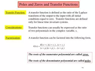
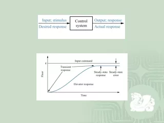
Out response, Poles, and Zeros • The output response of a system is the sum of two responses: the forced response (steady-state response) and the natural response (zero input response) • The poles of a transfer function are (1) the values of the Laplace transform variable, s , that cause the transfer function to become infinite, or (2) any roots of the denominator of the transfer function that are common to roots of the numerator. • The zeros of a transfer function are (1) the values of the Laplace transform variable, s , that cause the transfer function to become zero, or (2) any roots of the numerator of the transfer function that are common to roots of the denominator.
Figure 4.1a. System showing input and output;b. pole-zero plot of the system;c. evolution of a system response.
A pole of the input function generates the form of the forced response. • A pole of the transfer function generates the form of the natural response. • A pole on the real axis generates an exponential response. • The zeros and poles generate the amplitudes for both the forced and natural responses.
Natural response Forced response
First-Order Systems Figure 4.4a. First-order systemb. pole plot Figure 4.5First-order systemresponse to a unit step
The time constant can be described as the time for to decay to 37% of its initial value. Alternately, the time is the time it takes for the step response to rise to of its final value. • The reciprocal of the time constant has the units (1/seconds), or frequency. Thus, we call the parameter the exponential frequency.
Rise time: Rise time is defined as the time for the waveform to go from 0.1 to 0.9 of its final value. • Settling time: Settling time is defined as the time for the response to reach, and stay within, 2% (or 5%) of its final value.
Second-Order Systems Figure 4.7Second-ordersystems, pole plots,and step responses
1. Overdamped response: Poles: Two real at Natural response: Two exponentials with time constants equal to the reciprocal of the pole location • 2. Underdamped responses: Poles: Two complex at Natural response: Damped sinusoid with and exponential envelope whose time constant is equal to the reciprocal of the pole’s real part. The radian frequency of the sinusoid, the damped frequency of oscillation, is equal to the imaginary part of the poles
3. Undamped response: Poles: Two imaginary at Natural response: Undamped sinusoid with radian frequency equal to the imaginary part of the poles • 4. Critically damped responses: Poles: Two real at Natural response: One term is an exponential whose time constant is equal to the reciprocal of the pole location. Another term is the product of time and an exponential with time constant equal to the reciprocal of the pole location
Figure 4.10Step responses for second-ordersystem damping cases
Figure 4.8Second-order step response componentsgenerated by complex poles
Natural Frequency: The natural frequency of a second-order system is the frequency of oscillation of the system without damping. • Damping Ratio: The damping ratio is defined as the ratio of exponential decay frequency to natural frequency. Consider the general system: Without damping,
Figure 4.11Second-order response as a function of damping ratio
Underdamped Second-Order Systems Step response Taking the inverse Laplace transform where
Figure 4.13Second-order underdampedresponses for damping ratio values
Peak time: The time required to reach the first, or maximum, peak. • Percent overshoot: The amount that the waveform overshoots the steady-state, or final, value at the peak time, expressed as a percentage of the steady-state value. • Settling time: The time required for the transient’s damped oscillations to reach and stay within (or ) of the steady-state value. • Rise time: The time required for the waveform to go from 0.1 of the final value to 0.9 of the final value. Evaluation of peak time: Setting the derivative equal to zero yields Peak time:
Evaluation of percent overshoot ( ): Evaluation of settling time: The settling time is the time it takes for the amplitude of the decaying sinusoid to reach o.o2, or , where is the imaginary part of the pole and is called the damped frequency of oscillation, and is the magnitude of the real part of the pole and is the exponential damping frequency.
Figure 4.18Lines of constant peak time,Tp , settlingtime,Ts , and percent overshoot, %OSNote: Ts2 < Ts1 ;Tp2 < Tp1; %OS1 <%OS2
Figure 4.19Step responses of second-orderunderdamped systems as poles move:a. with constant real part;b. with constant imaginary part;c. with constant damping ratio
Find peak time, percent overshoot, and settling time from pole location. , ,
Figure 4.21Rotational mechanical system Design: Given the rotational mechanical system, find J and D to yield 20% overshoot and a settling time of 2 seconds for a step input of torque T(t).
Under certain conditions, a system with more than two poles or with zeros can be approximated as a second-order system tat has just two complex dominant poles. Once we justify this approximation, the formulae for percent overshoot, settling time, and peak time can be applied to these higher-order systems using the location of the dominant poles. Figure 4.23Component responses of a three-pole system:a. pole plot;b. component responses: nondominant pole is near dominant second-order pair (Case I), far from the pair (Case II), and at infinity (Case III) Remark: If the real pole is five times farther to the left than the dominant poles, we assume that the system is represented by its dominant second-order pair of poles.
Figure 4.25Effect of addinga zero to a two-pole system System response with zeros If the zero is far from the poles, then is large comared to and .
Time Domain Solution of State Equations where is called the state-transition matrix.