Dynamic Systems: Transfer Functions and Control Design
130 likes | 190 Vues
Explore the concepts of Transfer Functions, Poles, and Zeros in Dynamic Systems. Learn how to manipulate system stability and response through control design techniques like pole placement. Dive into intricate calculations and practical applications.

Dynamic Systems: Transfer Functions and Control Design
E N D
Presentation Transcript
MEM 351 – Dynamic Systems Lab Representations: Transfer Functions Poles and Zeros
Recall Bar length [m] Pivot to CG distance [m] Mass of pendulum [kg] Moment of Inertia Viscous damping coefficient Damped Compound Pendulum Equations of Motion Linearized 2nd order differential equation assumes small angles General 2nd order form
Tedious Math: Time domain differential equation 2nd order damped system Yields complex roots Time domain solution (1) Small real root will yield long settling times Can be shown: (2) Time constant 2% settling time
Easier Math I: Laplace Domain • Voltage applied to motor • Propeller spins, creating lift force • Lift on lever arm r creates torque • Pendulum rotates angle
Calculating Constants Theory: can calculate lift force if have propeller pitch and radius dimensions, air density and motor angular velocity. Experimentally, apply known voltage V and pendulum will eventually reach steady-state. Recall At steady-state angular acceleration and velocity are zero. The torque at this known voltage is calculated by: And hence
Open-Loop Transfer Function OLTF: Given Nm/V m 2 (3) kgm kg Nms/rad Laplace domain OL Transfer function
OLTF Simulations Simulink
Roots of the denominator (i.e. the poles) are: Small real root will yield long settling times Simulation reveals long settling time. This is consistent with the low viscous damping coefficient. Poles of the characteristic equation reveal the large oscillations. Recall from (1) In other words, the system is bordering on the margin of stability. Recall Equations (1) and (2).
Control Designer’s Goal: (1) Create compensators that yield desired damping and rise time. (2A) In other words, place poles where one wants them (2B) System Poles and Zeros – What are they?
Calculated the following: rad/s poles
Poles are the roots of the characteristic equation. As such, the describe stability through and Where are we going with this? It’s called the characteristic equation because it connotes system properties Question: can we alter the locations of the poles? If we can, then we change the characteristic of the system… Answer: This is exactly what the control engineer does. One popular method is called “pole placement” control