Z-Transform.
CHAPTER 5. Z-Transform. EKT 230. 5.0 Z-Transform. 5.1 Introduction. 5.2 The z-Transform. 5.2.1 Convergence. 5.2.2 z-Plane. 5.2.3 Poles and Zeros. 5.3 Properties of Region of Converges (ROC). 5.4 Properties of z-Transform. 5.5 Inverse of z-Transform. 5.6 Transfer Function.


Z-Transform.
E N D
Presentation Transcript
CHAPTER 5 Z-Transform. EKT 230
5.0 Z-Transform. 5.1 Introduction. 5.2 The z-Transform. 5.2.1 Convergence. 5.2.2 z-Plane. 5.2.3 Poles and Zeros. 5.3 Properties of Region of Converges (ROC). 5.4 Properties of z-Transform. 5.5 Inverse of z-Transform. 5.6 Transfer Function. 5.7 Causality and Stability. 5.8 Discrete and Continuous Time Transformation. 5.9 Unilateral z-Transformation.
Relation to the Laplace Transform • The z transform is to discrete-time signals and systems what the Laplace transform is to continuous-time signals and systems
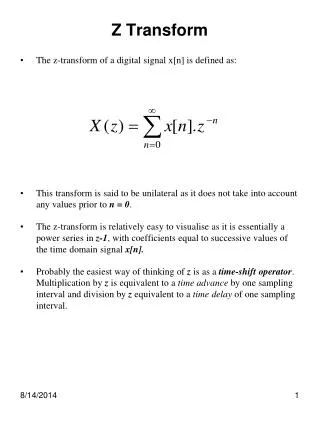
Definition The definition of the z transform of a discrete-time function x is and x and X form a “z-transform pair”
5.2.2 z-Plane. Figure 5.3: The unit circle, z = ej, in the z-plane. • It is convenience to represent the complex frequency z as a location in z-plane as shown in Figure 5.2. Figure 5.2: The z-plane. A point z = rej is located at a distance r– from the origin and an angle relative to the real axis. • The point z=rej Wis located at a distance r from the origin and the angle W from the positive real axis. • Figure 5.3 is a unit circle in the z-plane. z=rej Wdescribes a circle of unit radius centered on the origin in the z-plane.
5.4 Properties of z-Transform. • Most properties of z-transform are similar to the DTFT. We assumed that, • The effect of an operation on the ROC is described by a change in the radii of the ROC boundaries. (1) Linearity,
Cont’d… (2) Time Reversal. (3) Time Shift. with ROC Rx, except possibly z=0 or |z|= infinity.
Cont’d… (4) Multiplication by an Exponential Sequence. (5) Convolution. (6) Differentiation in the z-Domain.
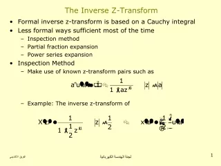
5.5 The Inverse Z-Transform. • There are two common methods; 5.5.1 Partial-Fraction Expression. 5.5.2 Power-Series Expansion.
5.5.1 Partial-Fraction Expansion. Example 5.1:Inversion by Partial-Fraction Expansion. Find the inverse z-transform of, with ROC 1<|z|<2. Figure 5.6: Locations of poles and ROC. Solution: Step 1:Use the partial fraction expansion of Z(s) to write Solving the A, B and C will give
Cont’d… Step 2:Find the Inverse z-Transform for each Terms. - The ROC has a radius greater than the pole at z=1/2, it is the right-sided inverse z-transform. - The ROC has a radius less than the pole at z=2, it is the left-sided inverse z-transform. - Finally the ROC has a radius greater than the pole at z=1, it is the right-sided inverse z-transform.
Cont’d… Step 3: Combining the Terms. • .
Example 5.2:Inversion of Improper Rational Function. Find the inverse z-transform of, with ROC |z|<1. Figure 5.7: Locations of poles and ROC. Solution: Step 1: Convert X(z) into Ratio of Polynomial in z-1. Factor z3 from numerator and 2z2 from denominator.
Step 2: Use long division to reduce order of numerator polynomial. Factor z3 from numerator and 2z2 from denominator.
Factor z3 from numerator and 2z2 from denominator. We define, Where, With ROC|z|<1 Step 3:Find the Inverse z-Transform for each Terms. • .
5.6 Transfer Function. • The transfer function is defined as the z-transform of the impulse response. y[n]= h[n]*x[n] • Take the z-transform of both sides of the equation and use the convolution properties result in, • Rearrange the above equation result in the ratio of the z-transform of the output signal to the z-transform of the input signal. • The definition applies at all z in the ROC of X(z) and Y(z) for which X(z) is nonzero.
Example 5.3:Find the Transfer Function. Find the transfer function and the impulse response of a causal LTI system if the input to the system is Solution: Step 1: Find the z-Transform of the input X(z) and output Y(z). With ROC |z|>1/3 With ROC |z|>1.
Step 2: Solve for H(z). , with ROC |z|>1. Solve for impulse response h[n], , with ROC |z|>1. So the impulse response h[n] is, • .
5.7 Causality and Stability. Figure 5.8: Pole and impulse response characteristic of a causal system. (a) A pole inside the unit circle contributes an exponentially decaying term to the impulse response. (b) A pole outside the unit circle contributes an exponentially increasing term to the impulse response. • The impulse response of a causal system is zero for n<0. • The impulse response of a casual LTI system is determined from the transfer function by using right-sided inverse transform. • The poles inside the unit circle, contributes an exponentially decaying term to the impulse response. • The poles outside the unit circle, contributes an exponentially increasing term.
Cont’d… Figure 5.9: Pole and impulse response characteristics for a stable system. (a) A pole inside the unit circle contributes a right-sided term to the impulse response. (b) A pole outside the unit circle contributes a left-sided term to the impulse response. • Stable system; the impulse response is absolute summable and the DTFT of impulse response exist. • The impulse response of a casual LTI system is determined from the transfer function by using right-sided inverse transform. • The poles inside the unit circle, contributes a right-sided decaying exponential term to the impulse response. • The poles outside the unit circle, contributes a left-sided decaying exponentially term to the impulse response. • Refer to Figure 5.9.
Cont’d… Figure 7.16: A system that is both stable and causal must have all its poles inside the unit circle in the z-plane, as illustrated here. Stable/Causal ? • From the ROC below the system is stable, because all the poles within the unit circle and causal because the right-sided decaying exponential in terms of impulse response.
5.8 Implementing Discrete-Time LTI System. • The system is represented by the differential equation. • Taking the z-transform of difference equation gives, • The transfer function of the system,
5.9 The Unilateral z-Transform. • The unilateral z-Transform of a signal x[n] is defined as, Properties. • If two causal DT signals form these transform pairs, (1) Linearity. (2) Time Shifting.