The z -Transform
The z -Transform. The representation for a sampled function was shown to be. Taking the Laplace transform of this function we have. If we let z=e sT , we have.


The z -Transform
E N D
Presentation Transcript
The representation for a sampled function was shown to be Taking the Laplace transform of this function we have
If we let z=esT,we have The samples in the sum are multiplied by z-n. Each factor z-n corresponds to a factor of e-snT in Laplace domain. Multiplying by e-snT in Laplace domain corresponds to a delay in time domain:
Example: Find the z-transform of the discrete-time step function u[n] n 1 2 3 4 5
By simply inserting this discrete-time function into the definition of the z-transform, we have
To evaluate this sum, we use the formula for an infinite geometric series: This summation converges to the above expression if |a|<1. A derivation of this expression is on the following slide.
Using the formula for the infinite geometric series the z-transform of the unit step function is
Since z is a complex number, this last statement is equivalent to those values of z whose magnitude is greater than one: or,
The region corresponds to a circle in the complex plane. (zr is like x and zi is like y.) Thus, the region is the region exteriorto the unit circle.
Im{z} Re{z}
Im{z} Re{z}
Example: Find the z-transform of -u[-n-1] -1 -3 -2 n 1 2 3 4 5
In this case, we have an anticausalfunction. Strictly speaking, it is impossible to generate this function, but it may arise as a solution to a design. Such functions correspond to nonrealizable systems. The z-transform of this function will be a sum like the z-transform for the step function, but the index will be negative:
We see that the z-transform of the anticausal step function is the same as that of the ordinary step function. This z-transform converges for |z|<1 (look at the last summation before the geometric series formula is applied). The region |z|<1 corresponds to
Im{z} Re{z}
Example: Find the z-transform of a discrete-time exponential function where |a| < 1. anu[n] n 1 2 3 4 5
To find the z-transform, we proceed in much the same fashion as we did before:
The region of convergence is |az-1 | < 1, or |z|>a. Notice that the regions of convergence do not contain any of the poles of the z-transform. The poles are where the denominator is zero. For the unit step function z-transform, the pole was at z=1. For anun, the pole is at z=a. Poles are marked with an ‘x’.
Im{z} Re{z}
Example: Find the z-transform of a discrete-time ramp function r[n] n 1 2 3 4 5
The first step in finding this z-transform is the same as with other z-transforms: To proceed from here, we need to use a small trick:
The last expression is the term inside the sum of the z-transform of the ramp multiplied by z. So if we multiply the transform by z-1z, we have
The region of convergence is the same as that for the unit step function: |z|>1.
Example: Find the z-transform of a discrete-time impulse function d[n] n -2 -1 1 2 3
When evaluating the z-transform for this function, we see that only the n=0 term is non-zero A summary of the z-transforms of the causal signals is shown in the table on the following slide.
There are certain general characteristics that apply to all z-transforms. For example, if we multiply a z-transform by z-1, we achieve a delay in time-domain:
(In the last step, we substituted n-1 for n.) So, This property is perhaps the most important property of z-transforms.
In (continuous-time) linear system theory, we described the input/output relationship of a system by the following diagram:
We can find the output y(t) from the input x(t) by either using convolution with the impulse response or by multiplication by the transfer function in Laplace domain. Does a similar diagram exist for discrete-time functions?
To see if such relationships exist, let’s look at the bottom half of this diagram where we multiply X(z) by H(z) to get Y(z). By applying the definition of the z-transform, we can see what the equivalent (discrete-) time relationship would be.
Since we must necessarily have
This last expression is that of a discrete-time convolution:
Example: Find the discrete-time convolution of the following two functions: x[n] 2 1 n -2 -1 1 2 3 4 h[n] 1 n -2 -1 1 2 3 4
We start by evaluating the terms in the summation: x[m] and h[n-m] for various values of n. x[m] 2 1 m -2 -1 1 2 3 4 h[-m] n=0 1 m -2 -1 1 2 3 4
h[1-m] n=1 1 m -2 -1 1 2 3 4 h[2-m] n=2 1 m -2 -1 1 2 3 4 h[3-m] n=3 1 m -2 -1 1 2 3 4
We then find the sum of the products of the two functions. x[m] 2 1 m -2 -1 1 2 3 4 h[-m] n=0 1 m -2 -1 1 2 3 4
The values marked in red indicate values in both functions whose product is notzero. Non-red values will have a zero product. So from the red values we have Proceeding for n=1,2,…, we have
x[m] n=1 2 1 m -2 -1 1 2 3 4 h[1-m] 1 m -2 -1 1 2 3 4
x[m] n=2 2 1 m -2 -1 1 2 3 4 h[2-m] 1 m -2 -1 1 2 3 4
x[m] n=3 2 1 m -2 -1 1 2 3 4 h[3-m] 1 m -2 -1 1 2 3 4
So we have the following values for y[n]: The values for y[n] are zero for other values of n (n<0, n>3).
y[n] 3 2 1 n -2 -1 1 2 3 4
The same result could have been achieved using z-transforms: