Download
1 / 19
210 likes | 595 Vues
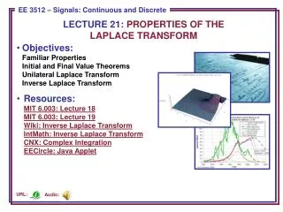
LECTURE 34: PROPERTIES OF THE Z-TRANSFORM AND THE INVERSE Z-TRANSFORM. Objectives: Modulation, Summation, Convolution Initial Value and Final Value Theorems Inverse z-Transform by Long Division Inverse z-Transform by Partial Fractions Difference Equations

E N D
LECTURE 34: PROPERTIES OF THE Z-TRANSFORMAND THE INVERSE Z-TRANSFORM • Objectives:Modulation, Summation, ConvolutionInitial Value and Final Value TheoremsInverse z-Transform by Long DivisionInverse z-Transform by Partial FractionsDifference Equations • Resources:MIT 6.003: Lecture 23Wiki: Inverse Z-TransformCNX: Inverse Z-TransformArslan: The Inverse Z-TransformCNX: PropertiesISIP: Pole/Zero Demo Audio: URL:
Properties of the z-Transform • Linearity: • Time-shift: • Multiplication by n: • Proof: • Multiplication by an: • Proof: • Multiplication by ejn: • Multiplication by cosn: • Multiplication by sinn: • Summation:
Convolution • Convolution: • Proof: • Change of index on the second sum: • The ROC is at least the intersection of the ROCs of x[n] and h[n], but can be a larger region if there is pole/zero cancellation. • The system transfer function is completely analogous to the CT case: • Causality: • Implies the ROC must be the exterior of a circle and include z =.
Initial-Value and Final-Value Theorems (One-Sided ZT) • Initial Value Theorem: • Proof: • Final Value Theorem: • Example: • Tables 7.2 and 7.3 in the textbook contain a summary of the z-Transform properties and common transform pairs.
Inverse Laplace Transform • Recall the definition of the inverse Laplace transform via contour integration: • The inverse z-transform follows from this: • Evaluation of this integral is beyond the scope of this course. Instead, as with the Laplace transform, we will restrict our interest in the inverse transform to rational forms (ratio of polynomials). We will see shortly that this is convenient since linear constant-coefficient difference equations can be converted to polynomials using the z-transform. • As with the Laplace transform, there are two common approaches: • Long Division • Partial Fractions Expansion • Expansion by long division Is also known as the power series expansion approach and can be easily demonstrated by an example.
Long Division • Consider: • Solution: Implications of stability?
Inverse z-Transform Using MATLAB • Consider: • MATLAB: • Syms X x z • X = (8*z^3+2*z^2-5*z)/(z^3-1.75*z+.75); • x = iztrans(X) • x = 2*(1/2)^n+2*(-3/2)^n+4 • Evaluate numerically: • num = [8 2 -5 0]; • den = [1 0 -1.75 .75]; • x = filter(num, den, [1 zeros(1,9)]) • Output: • 8 2 9 -2.5 14.25 -11.125 26.8125 -30.1563 55.2656
Inverse z-Transform Using Partial Fractions • Rational transforms can be factored using the same partial fractions approach we used for the Laplace transforms. • The partial fractions approach is preferred if we want a closed-form solution rather than the numerical solution long division provides. • Example: • In this example, the order of the numerator and denominator are the same. For this case, we can use a trick of factoring X(z)/z:
Inverse z-Transform (Cont.) We can compute the inverse using our table of common transforms: The exponential terms can be converted to a single cosine using a magnitude/phase conversion:
Inverse z-Transform (Cont.) • This can be verified using MATLAB: • num = [1 0 0 1]; • den = [1 -1 -1 -2 0]; • [r, p] = residue(num, den) • r = p= • 0.6429 2.0000 • 0.4286 – 0.825i -0.5000 + 0.8660i • 0.4286 + 0.825i -0.5000 – 0.8660i • -0.5000 0 • The first 20 samples of the output can be computed numerically using: • num = [1 0 0 1]; • den = [1 -1 -1 -2 0]; • x = filter(num, den, [1 zeros(1,19)]); • Using MATLAB as a resource for solving homework problems can greatly reduce the time you spend doing busywork.
First-Order Difference Equations • Consider a first-order difference equation: • We can apply the time-shift property: • We can solve for Y(z): • The response is again a function of two things: the response due to the initial condition and the response due to the input. • If the initial condition is zero: • Applying the inverse z-Transform: • Is this system causal? Why? • Is this system stable? Why? • Suppose the input was a sinusoid. How would you compute the output?
Example of a First-Order System • Consider the unit-step response of this system: • Use the (1/z) approach for the inverse transform: • The output consists of a DC term, an exponential term due to the I.C., and an exponential term due to the input. Under what conditions is the output stable?
Second-Order Difference Equations • Consider a second-order difference equation: • We can apply the time-shift property: • Assume x[-1] = 0 and solve for Y(z): • Multiplying z2/z2: • Assuming the initial conditions are zero: • Note that the impulse response is of the form: • This can be visualized as a complex pole pair with a center frequency and bandwidth (see Java applet).
Example of a Second-Order System • Consider the unit-step response of this system: • We can further simplify this: • The inverse z-transform gives: MATLAB: num = [1 -1 0]; den = [1 1.5 .5]; n = 0:20; x = ones(1, length(n)); zi = [-1.5*2-0.5*1, -0.5*2]; y = filter(num, den, x, zi);
Nth-Order Difference Equations • Consider a general difference equation: • We can apply the time-shift property once again: • We can again see the important of poles in the stability and overall frequency response of the system. (See Java applet). • Since the coefficients of the denominator are most often real, the transfer function can be factored into a product of complex conjugate poles, which in turn means the impulse response can be computed as the sum of damped sinusoids. Why? • The frequency response of the system can be found by setting z =ej.
Transfer Functions • In addition to our normal transfer function components, such as summation and multiplication, we use one important additional component: delay. • This is often denoted by its z-transform equivalent. • We can illustrate this with an example (assumeinitial conditions are zero): z-1 D
Transfer Function Example • Redraw using z-transform: • Write equations for the behavior at each of the summation nodes: • Three equations and three unknowns: solve the first for Q1(z) and substitute into the other two equations.
Summary • Introduced additional properties of the z-transform. • Derived the convolution property for DT LTI systems. • Introduced two practical ways to compute the inverse z-transform: long division and partial fractions expansion. • Worked examples of each and demonstrated how to solve these problems using MATLAB. • Demonstration: Frequency response using a Java applet that allows you to visualize poles and zeros in the complex plane. • Demonstrated the solution of Nth-order difference equations using thez-transform: general response is an exponential. • Demonstrated how to develop and decompose signal flow graphs using the z-transform: introduced a component, the delay, which is equivalent to differentiation in the s-plane.