Download
1 / 11
150 likes | 646 Vues
LECTURE 21: PROPERTIES OF THE LAPLACE TRANSFORM. Objectives: Familiar Properties Initial and Final Value Theorems Unilateral Laplace Transform Inverse Laplace Transform

E N D
LECTURE 21: PROPERTIES OF THELAPLACE TRANSFORM • Objectives:Familiar PropertiesInitial and Final Value TheoremsUnilateral Laplace TransformInverse Laplace Transform • Resources:MIT 6.003: Lecture 18MIT 6.003: Lecture 19Wiki: Inverse Laplace TransformIntMath: Inverse Laplace TransformCNX: Complex IntegrationEECircle: Java Applet Audio: URL:
Familiar Properties of Linear Transforms • To introduce the inverse Laplace transform and some important applications of the transform (e.g., circuits), we will need to introduce some familiar properties of the transform (e.g., linearity). • There are some properties unique to the Laplace transform (e.g., the Initial Value Theorem). • There are some properties of the Fourier Transform that do not have an equivalent for the Laplace transform (e.g., duality, Parseval’s theorem). • Linearity: • Note that the ROC for the sum is at least the intersection of the ROCs for each component (it must include regions for which both transforms converge, as we demonstrated in lecture 21). • In some special cases, the ROC can be larger (e.g., when the zeroes of one component cancel the poles of the other component). For example: • Example:
Properties of the Laplace Transform • Time-Shift: • Example: • Note that the ROC doesn’t change because it is defined by the pole location. • Example: • What is the ROC? Hint: This is a time-limited signal. • Time Scaling: • Example: • Is this result expected?
More Properties • Multiplication by a Power of t: • Compare to Fourier transform: • Example: • Time-Domain Differentiation (Bilateral): • Example: • Integration:
Convolution • The convolution integral: • Laplace transform is analogous to the Fourier transform: • But, because the Laplace transform and its inverse (to be discussed in a moment) are not symmetric, the dual of this is not true: • This is one reason the Fourier transform is more popular for applications involving communications systems and modulation. • The ROC is at least the overlap of the ROCs for each signal (again, it can be larger than the ROC for either signal). • Example: CT LTI
The Unilateral (One-sided) Laplace Transform • Define a special case of the Laplacetransform for right-sided signals: • For right-sided signals ( ), and for causal systems ( ), the one-sided and two-sided transforms are equal. • Several properties change slightly, such as differentiation: • Proof: • Other properties, such as convolution, hold as is, as long as the system is causal and the input starts at t = 0.
Initial and Final Value Theorems • Theorem: • Proof: • Applying the differentiation property: • The initial value theorem can be extended to higher-order derivatives: • Allow initial and final conditions to be computed directly from the transform.
Application of the Initial and Final Value Theorems • Consider a rational transform: • Initial value: • For example: • Final Value:
Inverse Laplace Transform using Complex Integration • Recall: • Choose ROC and apply the inverse Fourier transform: • But for a fixed , s = + j, ds = j d: • This is a contour integral in the complex plane. Such integrals are studied extensively in a course on complex variables, but are beyond the scope of this course.
Specific Cases of Inverse Laplace Transforms • We will restrict ourselves to two special case: • Rational transforms: use partial fractions expansion • Exponentials: use the shift property: • These two building blocks will allow us to construct the inverse transforms for many common signals and systems, including those used in circuit analysis. • Therefore, the unilateral Laplace transform can be applied to finding both the transient and steady-state responses (as well as the frequency response) of a circuit. This is one of its principal uses in electrical engineering. • The use of partial fractions, however, requires being able to factor a polynomial into its roots. You have previously used this in calculus, and have good MATLAB support for this as well.
Summary • Review your tables of transform properties (one-sided!) and common transform pairs: