Chapter 6 z-Transform

1. Chapter 6 z-Transform Definition ROC (Region of Converges) z-Transform Properties Transfer Function

2. frequency domain --a sequence in terms of complex exponential sequences of the form { }; The Discrete-time signals can be represented in: • time domain --a weighted linear combination of delayed unit sample sequences; • Z domain --a sequence in terms of complex exponential sequences of the form{ Z-n }.

3. Why need z-Transform? • The DTFT provides a frequency-domain representation of discrete-time signals and LTI discrete-time systems; • Because of the convergence condition, in many cases, the DTFT of a sequence may not exist; • As a result, it is not possible to make use of such frequency-domain characterization in these cases.

4. Why need z-Transform? • A generalization of the DTFT leads to the z-transform. z-transform may exist for many sequences for which the DTFT does not exist. For a real-valued sequence, the z-transform is a real-rational function of complex variable z. Moreover, use of z-transform techniques permits simple algebraic manipulations.

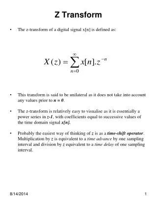
5. 6.1 Definition and Properties • For a given sequence g[n], its z-transform G(z) is defined as: where z = Re(z) + jIm(z) is a complex variable.

6. If we let z = rej, then the z-transform reduces to: • For r = 1 (i.e., |z| = 1), z-transform reduces to its DTFT, provided the latter exists; • The contour |z| = 1 is a circle in the z-plane of unity radius and is called the unit circle.

7. Like the DTFT, there are conditions on the convergence of the infinite series For a given sequence, the set R of values of z for which its z-transform converges is called the region of convergence (ROC) ★

8. From our earlier discussion on the uniform convergence of the DTFT, it follows that the series converges if {g[n]r-n} is absolutely summable, i.e., if

9. In general, the ROC of a z-transform of a sequence g[n] is an annular region of the z-plane: where Note: The z-transform is a form of a Laurent series and is an analytic function at every point in the ROC.

10. Example: Determine the z-transform X(z) of the causal sequence x[n]=n[n] and its ROC. The above power series converges to ROC is the annular region |z| > |a|

11. m ROC is the annular region • The z-transform m(z) of the unit step sequence m[n] can be obtained from by setting a = 1: • Note: u[n] is not absolutely summable, and hence its DTFT does not converge uniformly.

12. ROC is the annular region • Example: Consider the anti-causal sequence: Its z-transform is given by:

13. Note: The z-transforms of the two sequences n[n] and -n[-n-1]are identical even though the two parent sequences are different. • Only way a unique sequence can be associated with a z-transform is by specifying its ROC.

14. The DTFT G(ej) of a sequence g[n] converges uniformly if and only if the ROC of the z-transform G(z) of g[n] includes the unit circle. • The existence of the DTFT does not always imply the existence of the z-transform.

15. Example - The finite energy sequence has a DTFT given by It converges in the mean-square sense. • However, hLP[n] does not have a z-transform as it is not absolutely summable for any value of r.

16. Table6.1 Commonly Usedz-transform

17. 6.2 Rationalz-transform • In the case of LTI discrete-time systems we are concerned with in this course, all pertinent z-transforms are rational functions of z-1 • That is, they are ratios of two polynomials in z-1 :

18. The degree of P(z) is M and the degree of D(z) is N; • An alternate representation of a rational z-transform is as a ratio of two polynomials in z:

19. A rational z-transform can be alternately written in factored form as • z=l , G(l) = 0 --- zeros of G(z); • z=l , G(l) --- poles of G(z).

20. m • Example: has a zero at z = 0 and a pole at z = 1:

21. A physical interpretation of the concepts of poles and zeros can be given by plotting the log-magnitude 20log10|G(z)| as shown on next slide for

22. poles z=0.4±j0.6928, zeros z=1.2±j1.2

23. 6.3 ROC of a Rational z-transform • ROC of a z-transform is an important concept. • Without the knowledge of the ROC, there is no unique relationship between a sequence and its z-transform. • Hence, the z-transform must always be specified with its ROC. • Moreover, if the ROC of a z-transform includes the unit circle, the DTFT of the sequence is obtained by simply evaluating the z-transform on the unit circle.

24. There is a relationship between the ROC of the z-transform of the impulse response of a causal LTI discrete-time system and its BIBO stability. • The ROC of a rational z-transform is bounded by the locations of its poles. • To understand the relationship between the poles and the ROC, it is instructive to examine the pole-zero plot of a z-transform.

25. Example: • The z-transform H(z) of the sequence h[n]=(-0.6)n[n] is given by • Here the ROC is just outside the circle going through the point z=-0.6

26. Example: • Consider a finite-length sequence g[n] defined for - MnN, where M and N are non-negative integers and |g(n)|<  • Its z-transform is given by: G(z) has M poles at z =  and N poles at z = 0

27. A sequence can be one of the following types: finite-length, right-sided, left-sided and two-sided. • In general, the ROC depends on the type of the sequence of interest. • As can be seen from the last example, the z-transform of a finite-length bounded sequence converges everywhere in the z-plane except possibly at z = 0 and/or at z =  .

28. A right-sided sequence with nonzero sample values for n0 is sometimes called a causal sequence. • Consider a causal sequence u1[n] • Its z-transform is given by:

29. It can be shown that U1(z) converges exterior to a circle |z|=R1, including the point z = . • On the other hand, a right-sided sequence u2[n] with nonzero sample values only for n ³ - M with M nonnegative has a z-transform U2(z) with M poles at z = . • The ROC of U2(z) is exterior to a circle |z|=R2, excluding the point z = .

30. A left-sided sequence with nonzero sample values for n0 is sometimes called a anticausal sequence. • Consider an anticausal sequence v1[n] • Its z-transform is given by:

31. It can be shown that V1(z) converges interior to a circle |z|=R3 , including the point z = 0. • On the other hand, a left-sided sequence with nonzero sample values only for nN with N nonnegative has a z-transform V2(z) with N poles at z = 0. • The ROC of V2(z) is interior to a circle |z|=R4 , excluding the point z = 0.

32. The first term: The z-transform of a two-sided sequence w[n] can be expressed as: can be interpreted as the z-transform of a right-sided sequence and it thus converges exterior to the circle |z|=R5;

33. The second term: can be interpreted as the z-transform of a left-sided sequence and it thus converges interior to the circle |z|=R6; • If R5 < R6 , there is an overlapping ROC given by R5 < |z| < R6 • If R5 > R6 , there is no overlap and the z-transform does not exist.

34. Example: • Consider the two-sided sequence: u[n] = n , where a can be either real or complex. • Its z-transform is given by: The first term converges for |z| > ||, whereas the second term converges for |z| < ||. • There is no overlap between these two regions; Hence, the z-transform of u[n] = n does not exist.

35. To show that the z-transform is bounded by the poles, assume that the z-transform X(z) has simple poles at z=α and z=β.

36. The ROC of a rational z-transform cannot contain any poles and is bounded by the poles. • In general, if the rational z-transform has N poles with R distinct magnitudes, then it has R+1 ROCs; • Thus there are R+1 distinct sequences with the same z-transform. • Hence, a rational z-transform with a specified ROC has a unique sequence as its inverse z-transorm.

37. MATLAB functions • The ROC of a rational z-transform can be easily determined using MATLAB [z, p, k] = tf2zpk(num, den) determines the zeros, poles, and the gain constant of a rational z-transform with the numerator coefficients specified by the vector num and the denominator coefficients specified by the vector den. • [num,den] = zp2tf(z, p, k) implements the reverse process.

38. k • The pole-zero plot is determined using the function zplane. • The z-transform can be either described in terms of its zeros and poles: zplane(zeros, poles) • or, it can be described in terms of its numerator and denominator coefficients: zplane(num,den)

39. %Find second-order factors [sos, g] = zp2sos(z,p,k) [sos, g] = tf2sos(b,a)

40. 2 1 Imaginary Part 0 -1 -2 -4 -3 -2 -1 0 1 Real Part • Example num = [2,16,44,56,32]; den = [3,3,-15,18,-12]; zplane(num,den); [z, p, k] = tf2zp(num, den); %zplane(z,p);

41. 6.4Inverse z-Transform • General Expression: Recall, for z=rej, the z-transform G(z) given by • is merely the DTFT of the sequence g[n]r-n • Accordingly, the inverse DTFT is thus given by

42. By making a change of variable z=rej, the previous equation can be converted into a contour integral given by where C’ is a counterclockwise contour of integration defined by |z| = r. • The contour integral can be evaluated using the Cauchy’s residue theorem resulting in:

43. 2. The calculation for inverse Z-Transform (1) Table Look-up Method (2) Partial Fraction Expansion (3) Long Division (1) Table Look-up Method Example 6.12 (p.314)

44. Partial-Fraction Expansion • A rational G(z) can be expressed as If MN then G(z) can be re-expressed as: where the degree of P1(z) is less than N. • The rational function P1(z)/D(z) is called a proper fraction.

45. Example - Consider Solution:

46. Simple Poles: In most practical cases, the rational z-transform of interest G(z) is a proper fraction with simple poles. • Let the poles of G(z) be at z=k, 1 k N • A partial-fraction expansion of G(z) is then of the form

47. The constants lin the partial-fraction expansion are called the residues and are given by Each term of the sum in partial-fraction expansion has an ROC given by |z|>|l| and, thus has an inverse transform of the form l(l)n[n]

48. Therefore, the inverse transform g[n] of G(z) is given by Note: The above approach with a slight modification can also be used to determine the inverse of a rational z-transform of a noncausal sequence.

49. Example - Let the z-transform H(z) of a causal sequence h[n] be given by A partial-fraction expansion of H(z) is then of the form

50. Now and