Random Rough Surface Scattering
z. y. x. PEC. Random Rough Surface Scattering . consider the rough surface scattering problem depicted above note that TM to z is equivalent to the TE case (transverse to the direction of propagation). z. y. x. PEC. Integral Equation. on the PEC surface. Integral Equation.

Random Rough Surface Scattering
E N D
Presentation Transcript
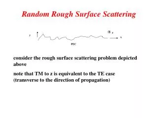
z y x PEC Random Rough Surface Scattering consider the rough surface scattering problem depicted above note that TM to z is equivalent to the TE case (transverse to the direction of propagation)
z y x PEC Integral Equation on the PEC surface
Integral Equation where f = y(x’)
Tapered Incident Field the rough surface has a finite length, is truncated at x=±L/2 the incident field cannot be a uniform plane wave, otherwise, diffraction from the end points may be significant the incident field is chosen as a tapered wave that reads g is the tapering parameter
Long Surface is Required for Near Grazing Incidence near grazing incidence, the RHS would not be close to zero g and therefore L must be very large for near grazing incidence
TE-to-z or TM (to the Direction of Propagation) Note that we can use the MFIE for the thin shell problem since a tapered wave is used, as the other side of the surface has zero fields.
Difference between TE and TM Case the former one has a symmetric impedance matrix while that of the latter one is non-symmetric when the surface is large, the number of unknowns will be large and the matrix solution time will be long we have developed a banded matrix iterative approach to solve a large matrix for the one-dimensional rough surface (a two-dimensional scattering) problem
Spatial Domain Methods one disadvantage of the spectral domain is that it requires numerical integration of infinite extend spatial domain Green’s functions are not readily available for layered media with applications in microstrip antennas and high-frequency circuits methods have been developed to circumvent this difficulty we will discuss the complex image method in conjunction with the Rao-Wilton-Glisson triangular discretization the mixed-potential integral equation (MPIE)
microstrip line W dielectric layer h Ѐr ground plane Microstrip Structures has arbitrary surface conductor geometry ground plane and substrate extend to infinity in the transverse direction and the space above the dielectric is unbounded the substrate is homogeneous and isotropic, but not necessarily lossless the upper conductor and ground plane have zero resistivity, and the upper conductor is infinitely thin our goal is to compute the surface current distribution from which other parameters can be extracted
Mixed-Potential Integral Equation (MPIE) it has weaker singularities in its Green’s functions than the EFIE, rendering more quickly convergent solutions
T- A- T+ A+ V- V+ Rao-Wilton-Glisson (RWG) Triangular Basis Functions O these functions overlap, and each plate can be part of up to three different basis functions
in in otherwise Rao-Wilton-Glisson (RWG) Triangular Basis Functions
Rao-Wilton-Glisson (RWG) Triangular Basis Functions the current flows from plate to , with maximum current across the common edge, zero current at the isolated vertices and , and no currents with components normal to the other four sides the weighting in the current representation is such that the current normal to the common edge is continuous across that edge, and hence, no fictitious charge singularities arise when the continuity equation is applied to the basis function, the charge density is a constant equal to and on each plate and the total charge is zero
Simplications many identical integrations will be performed considerable computational effort is saved by evaluating and storing the scalar potential integral for all plate combinations and recalling these results as needed in evaluating the matrix elements the same cannot be said of the integral for the vector potential, whose integrand evaluated over a particular source triangle depends on the identity of the isolated vertex and, hence, the basis function to which the triangle is assigned
Simplications where is set alternately to x’, y’and 1 the basis function dependence is removed from the integrals and reintroduced in the evaluation of Zmn through a weighted sum of these three for each plate combination, a total of four scalar integrals are evaluated and later recalled in constructing the elements in impedance matrix Z the excitation vector is given by
Spectral-Domain Green’s Function no closed-form expressions for Ga and Gq in the spatial domain, but they can be represented in closed-form in the spectral domain Wave numbers kzo and kr are the vertical and radial components of the free-space propagation constant ko in the cylindrical system RTE and RTM are the reflection coefficients at the interface of TE and TM plane waves incident on the substrate with ground plane
Spatial Green’s Function through Transformation the spatial-domain Green’s functions can then be expressed as an inverse Hankel-transform of the spectral counterparts, commonly referred to as Sommerfeld integrals Approximate analytic expressions exist for the evaluation of the Hankel-transform for r in the near and far fields a technique developed by Prof. Fang Dagang of the Nanjing University of Science and Technology and improved by Prof. Y. L. Chow allows efficient evaluation in all regions
Complex Image Method the Sommerfeld integral is divided into three contributions: 1) quasi-dynamic images, 2) surface waves, and 3) complex images the first two contributions, which dominate respectively in the near-and far-field, are extracted from RTE and RTM and handled analytically using the Sommerfeld Identity what remains in RTE and RTM is relatively well behaved and exhibits exponential decay for sufficiently large values of kr the remainder can be accurately approximated with a short series of exponentials terms, which are interpreted as complex images
Complex Image Method the exponents of the expansion are computed using Prony’s method or the matrix pencil method and the term weights then obtained through a least-square fit the inverse Hankel-transform of the exponentials can be performed analytically, again using the Sommerfeld Identity two to four expansion terms are appropriate, depending on the frequency particular care should be taken in determining the number for expansion terms of Gq since its contribution in the scalar potential is a second-order difference arising from the source pulse-doublet and the testing procedure
Efficient Implementation all elements in the impedance matrix can be computed from a linear combination of four scalar integrals evaluated for all source/test plate combinations the surface integration over the source plate can be replaced by evaluation of the integrand at the plate centroid
Efficient Implementation the difference between the distances from the three vertices of the source plate to the test plate centroid is under some set maximum level, say 20%, then that approximation is viable it makes sense to evaluate the Green’s functions with an interpolation table both Ga and Gq exhibit 1/r and log r singularities, so the table must begin at some minimum displacement ro governed by the interpolation scheme, the dominant 1/r singularity, and a maximum error criterion, say 1%
Efficient Implementation the interactions can be catalogued by stepping through each plate combination far-interactions are ignored, as they are too numerous to store and can be rapidly evaluated through the Ga and Gq for near interactions, the four scalar integrals are evaluated and catalogued subsequent plate combinations are then checked against the stored interactions and computed only if no equivalent interactions is available Two plate interaction integrals are equivalent if the x- and y-displacements of the test plate centroid from the source plate vertices are identical
Curve Fitting using Complex Exponentials it is unfortunate that brute force application of signal processing techniques would not yield satisfactory results in representing our functions
Quasi-Dynamic Contributions at very low frequency, , RTE and Rq can be reduced to the quasi-dynamic form given by
Quasi-Dynamic Contributions surface-wave contribution dominates in the far field