CMPE 259
270 likes | 467 Vues
CMPE 259. Sensor Networks Katia Obraczka Winter 2005 Topology Control. Announcements. What’s topology control?. What’s topology control?. When nodes are deployed, how do they organize into a network? Neighbor-discovery protocol. If neighborhood is sparse, use all neighbors.

CMPE 259
E N D
Presentation Transcript
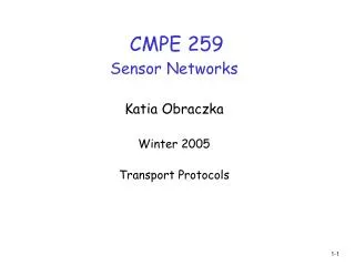
CMPE 259 Sensor Networks Katia Obraczka Winter 2005 Topology Control
What’s topology control? • When nodes are deployed, how do they organize into a network? • Neighbor-discovery protocol. • If neighborhood is sparse, use all neighbors. • What if neighborhood is dense? • Use a subset of neighbors. • How?
Approaches to topology control • Adjust transmit power. • Turn nodes on/off.
ASCENT: scenario • Ad hoc deployment. • Energy limitations. • Arbitrarily large scale. • Unattended operation. • Assume CSMA.
ASCENT: goals • Self-organization of nodes into topology that allows sensing coverage and communication under tight energy constraints.
ASCENT: approach • Nodes turn themselves on/off depending on assessment of operating conditions. • Neighborhood density. • Data loss.
State diagram After Tt Test Active Nbors<NT And Loss>LT or Help Nbors > NT or Loss > After Tp Passive Sleep After Ts
In “test” state: • Signaling (e.g., neighbor announcements). • After Tt, goes to “active”. • Or, if before Tt, number of neighbors>NT or average data loss (Tt) > average data loss (T0), go to “passive”.
In “passive” state: • After Tp, go to “sleep”. • If neighborhood is sparse loss > LT or “help” from “active” neighbor, go to “test”.
In “sleep”: • Turn off radio. • After Ts, go to “passive”.
In “active”: • Node does routing and forwarding. • Sends “help” if data loss > LT. • Stays on until runs out of battery!
Considerations • Why passive and test states? • Why once in active, a node runs until battery dies? • How to set parameters? • NT, LT. • Tt, Tp, Ts.
Neighborhood and loss • Node is neighbor if directly connected and link packet loss < NLS. • NLS is adjusted according to node’s number of neighbors. • Average loss date uses data packets only. • Packet is lost if not received from any neighbors.
Performance evaluation • Modeling, simulation, experimentation. • Metrics: • Packet loss. • Delivery ratio. • Energy efficiency. • Lifetime. • Time till 90% of transit nodes die.
Results • From the paper…
PEAS • Probing Environment, Adaptive Sleeping. • “Extra” nodes are turned off. • Nodes keep minimum state. • No need for neighborhood-related state. • PEAS consiers very high node density and failures are likely to happen.
Bi-modal operation • Probing environment. • Adaptive sleeping.
PEAS state diagram Working No reply for probe Wakes up Probing Sleeping Hears probe reply.
Probing • When node wakes up, enters probing mode. • Is there working node in range? • Broadcasts PROBE to range Rp. • Working nodes send REPLY (randomly scheduled). • Upon receiving REPLY, node goes back to sleep. • Adjusts sleeping interval accordingly. • Else, switches to working state.
Considerations • Probing range is application-specific. • Robustness (sensing and communication) versus energy-efficiency. • Location-based probing as a way to achieve balance between redundancy and energy efficiency. • Randomized sleeping time. • Better resilience to failure. • Less contention. • Adaptive based on “desired probing rate”.
More considerations… • Multiple PROBEs (and multiple REPLIES) to compensate for losses. • Multiple PROBEs randomly spread over time. • Multiple working nodes in the neighborhood. • Favor “oldest” one. • Nodes with fixed transmit power. • Deployment density.
Evaluation • Simulations. • Simulated failures: failure rate and failure percentage. • Metrics: • Coverage lifetime. • Delivery lifetime.
Results • With and without failures. • From the paper…