Fuzzy Models for Pattern Recognition Def.:

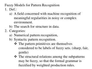
1. Fuzzy Models for Pattern Recognition • Def.: • A field concerned with machine recognition of meaningful regularities in noisy or complex environment. • The search for structure in data. • Categories: • Numerical pattern recognition, • Syntactic pattern recognition. • The pattern primitives are themselves considered to be labels of fuzzy sets. (sharp, fair, gentle) • The structural relations among the subpatterns may be fuzzy, so that the formal grammar is fuzzified by weighted production rules.

3. Elements of a numerical pattern recognition system: • Process description: data space →pattern space • Data: drawn from any physical process or phenomenon. • Pattern space (structure): the manner in which this information can be organized so that relationships between the variables in the process can be identified. • Feature analysis: feature space • Feature space has a much lower dimension than the data space.→essential for applying efficient pattern search technique. • Searches for internal structure in data items. That is, for features or properties of the data which allow us to recognize and display their structure.

4. Cluster analysis: search for structure in data sets. • Classifier design: classification space. • Search for structure in data spaces. • A classifier itself is a device, means, or algorithm by which the data space is partitioned into c decision regions.

5. Fuzzy Clustering • There is no universally optimal cluster criteria: distance, connectivity, intensity, … • Hierarchical clustering • Generate a hierarchy of partitions by means of a successive merging or splitting of clusters. • Can be represented by a dendogram, which might be used to estimate an appropriate number of clusters for other clustering methods. • On each level of merging or splitting a locally optimal strategy can be used, without taking into consideration policies used on preceding levels. • The methods are not iterative; they cannot change the assignment of objects to clusters made on proceeding levels. • Advantage: conceptual and computational simplicity. • Correspond to the determination of similarity trees.

8. Graph-theoretic clustering • Based on some kind of connectivity of the nodes of a graph representing the data set. • The clustering strategy is often breaking edges in a minimum spanning tree to form subgraphs. • Fuzzy data set →fuzzy graph. • Let G = [V,R] be a symmetric fuzzy graph. Then the degree of a vertex v is defined as d(v) = ∑u/=vμR(u,v). The minimum degree of G is δ(G) = min v∈V{d(v)}.

11. Let G be a symmetric fuzzy graph. G is said to be connected if, for each pair of vertices u and v in V, G is called Connected for some And G is connected. • Let G be a symmetric fuzzy graph. Clusters are then Defined as maximal Connected subgraph of G. • Objective-function clustering • The most precise formulation of the clustering criterion. • Local extrema of the objective function are defined as optimal clusterings. • Bezdek’s c-means algorithm.

12. Objective-function clustering • The most precise formulation of the clustering criterion. • Local extrema of the objective function are defined as optimal clusterings. • Bezdek’s c-means algorithm. • Butterfly example. • Similarity measure: distance of two objects • d: X × X→R+ which satisfies • D(xk,x1) = dk1 ≧0 • dk1 = 0 <= => xk = x1 • dk1 = d1k • (xk,x1 are the points in the p-dimensional space.)

13. Clustering: • Each partition of the set X into crisp or fuzzy subsets Si(i = 1,….,c) can fully be described by an indicator function • Let X = {x1,…,xn} be any finite set. Vcn is the set of all real c X n matrixes, and 2≦c≦n is an integer. The matrix U = [uik] ∈ Vcn is called a crisp c-partition if it satisfies the following conditions: The set of all matrixes that satisfy these conditions is called Mc.

15. Let X = {x1,…,xn} be any finite set. Vcn is the set of all real c X n matrixes, and 2≦c≦n is an integer. The matrix U = [uik] ∈ Vcn is called a fuzzy-c partition if it satisfies the following conditions: The set of all matrixes that satisfy these conditions is called Mfc. • Cluster center: vi = (vi1, …,vip): represents the location of a cluster. • vector of all cluster centers v = (vi,…,vc).

16. Variance criterion: measures the dissimilarity between the points in a cluster and its cluster center by the Euclidean distance. minimize the sum of the variances of all variables j in each cluster i (sum of the squared Euclidean distances) For crisp c-partition:

17. For fuzzy c-partition:

18. Fuzzy c-means algorithm • Step1: Choose c and m. Initialize U0∈Mfc, set r= 0 • Setp2: Calculate the c fuzzy cluster centers {vr} by using • Ur from Eq. 1. • Setp3: Calculate the new membership U1+1 by using {vr} Step4: Calculate Set r = r+1 and Go to step2. IF ,stop.

23. Decision Making • Characterized by • A set of decision alternatives • (decision space; constraints); • A set of states of nature (state space); • Utility (objective ) function: orders the results according to their desirability. • Fuzzy decision model: Bellman and Zadeh [1970] • Consider a situation of decision making under certainty, in which the objective function as well as the constraints are fuzzy. • The decision can be viewed as the intersection of fuzzy constraints and fuzzy objective function.

24. The relationship between constraints and objective functions in a fuzzy environment is therefore fully symmetric, that is , there is no longer a difference between the former and the latter. • The interpretation of the intersection depends on the context. • Intersection (minimum): no positive compensation (trade-off) between the membership degrees of the fuzzy sets in question. • Union (max): leads to a full compensation for lower membership degrees. • Decision = Confluence of Goads and Constraints.

25. Neither the noncompensatory “and” (min, product, Yager-conjunction) nor the fully compensatory “or” (max, algebraic sum, Yager-disjunction) are appropriate to model the aggregation of fuzzy sets representing managerial decisions. • Def: Let μCi(x), i=1,… ,m, x∈X, be membership functions of constraints, defining the decision space and μGj(x), j=1,…,n, x∈X the membership functions of objective functions or goals. A decision is then defined by its membership function where denote appropriate, possibly context- dependent aggregators.

26. Individual decision making

27. Multiperson decision making • Difference with individual decision making • Each places a different ordering on the alternatives • Each have access to different information • n-person game theories: both • Team theories: the second • Group decision theories: the first.

28. Multiperson decision making • Individual preference ordering: • Social choice function: • The degree of group preference of xiover xj • procedure to arrive at the unique crisp ordering that constitutes the group choice.

29. Fuzzy Linear Programming • Classical model: maximize f(x) = cTx such that Ax≦b x≧0 with c,x∈Rn,b∈Rm,A∈Rmxn. • Modification for fuzzy LP: • Do not maximize or minimize the objective function; might want to reach some aspiration levels which might not even be definable crisply. “improve the present cost situation considerably” • The constraints might be vague: coefficients, relations • Might accept small violations of constraints but might also attach different degrees of importance to violations of different constraints.

30. Symmetric fuzzy IP: • Find x such that cTx≧z (aspiration level) Ax≦b x≧0 • The membership function of the fuzzy set “decision” the above model is μi(x) can be interpreted as the degree to which x satisfies the fuzzy unequality Bix≦di. • Crisp optimal solution:

31. Membership function: e.g., optimal solution: that is maximizeλ

32. such that → (λ,x0) → the maximum solution can be found by solving one crisp LP with only one more variable and one more constraint.

33. Multistage Decision Making • Task-oriented control belongs to such kind of decision-making problem • Fuzzy decision making  fuzzy dynamic programming  a decision problem regarding a fuzzy finite-state automaton • State-transition relation is crisp • Next internal state is also utilized as output.

34. zt xt S one-time storage zt+1 Ct At S one-time storage Ct+1

35. Multistage Decision Making • Fuzzy input states as constraints: A0, A1 • Fuzzy internal state as goal: CN • Principle of optimality: An optimal decision sequence has the property that whatever the initial state and initial decision are, the remaining decisions must constitute an optimal policy with the state resulting from the first decision.

36. Multistage Decision Making

37. Fuzzy LP with crisp objective function • Constraints: define the decision space in a crisp of fuzzy way. • Objective function: induce an order of the decision alternatives. • Problem: the determination of an extremum of a crisp function over a fuzzy domain. • Approaches: • The determination of the fuzzy set “decision.” • The determination of a crisp “maximizing decision by aggregating the objective function after appropriate transformations with the constraints.

38. Fuzzy “decision” • Decision space is (partially) fuzzy. • Compute the corresponding optimal values of the objective function for all α-level sets of the decision space. • Consider as the fuzzy set “decision” the optimal values of the objective functions with the degree of membership equal to the corresponding α-level of the solution space. • Crisp maximizing decision.

39. Fuzzy Multi Criteria Analysis • Problems can not be done by using a single criterion or a single objective function. • Multi Objective Decision Making: concentrates on continuous decision space. • Multi Attribute Decision Making: focuses on problems with discrete decision spaces.

40. MODM: also called vector-maximum problem Def.: maximized {Z(x)|x∈X} where Z(x) = (z1(x),…,zk(x)) is a vector-valued function of x∈Rn into Rk and X is the “solution space” Stage in vector-maximum optimization: • The determination of efficient solution • The determination of an optimal compromise solution Efficient solution: xa is an efficient solution if there is no xb∈X such that Zi(xb)≧zi(xa) I=1,…,k and Zi(xb)>zi(xa) for at least one i =1,…,k. Complete solution: the set of all efficient solutions. Example:

41. MADM: Def.: Let X = {xi | i = 1,…,n} be a set of decision alternatives and G = {gj | j = 1,…,m} a set of goals according to which the desirability of an action is judged. Determine the optimal alternative x0 with the highest degree of desirability with respect to all relevant goals gj. Stages: • The aggregation of the judgments with respect to all goals and per decision alternative. • The rank ordering of the decision alternatives according to the aggregated judgments.

42. Fuzzy MADM: Yager model: Let X = {xi | i = 1,…,n} be a set of decision alternatives. The goals are represented by the fuzzy sets Gj, j = 1,…,m. The importance (weight) of goal j is expressed by wj. The attainment of goal Gj by alternative xi is expressed by the degree of membership μGj(xj). The decision is defined as the intersection of all fuzzy goals, that is D = G1 ∩ G2 ∩…∩ Gm. The optimal alternative is defined as that achieving the highest degree of membership in D.

43. FUZZY IMAGE TRANSFORM CODING • Transform coding: a transformation, perhaps an energy-preserving transform such as the discrete cosine transform (DCT), converts an image to uncorrelated data, (keep the transform coefficients with high energy and discard the coefficients with low energy, and thus compress the image data.) • (HDTV) systems have reinvigorated the image-coding field. (TV images correlate more highly in the time domain than in the spatial domain. Such time correlation permits even higher compression than we can achieve with still image coding.)

44. Adaptive cosine transform coding [Chen, 1977] produces high-quality compressed images at the less than I-bit/pixel rate. • Classifies subimages into four classes according to their AC energy level and encodes each class with different bit maps. • Assigns more bits to a subimage if the subimage contains much detail (large AC energy), and less bits if it contains less detail (small AC energy). • DC energy refers to the constant background intensity in an image and behaves as an average. • AC energy measures intensity deviations about the background DC average. So the AC energy behaves as a sample-variance statistic.

45. X DCT Coding Decoding DCT-1 X, Subimage Classification Figure10.1 Block diagram of adaptive cosine transform coding.

47. Selection of quantizing fuzzy-set values • Use percentage-scaled values of Ti and Li scaled by the maximum possible AC power value. • Compute the maximum AC power Tmax form the DCT coefficients of the subimage filled with random numbers from 0 to 255. • Calculate the arithmetic average AC powers for each class.

48. ADAPTIVE FAM SYSTEMS FOR TRANSFORM CODING • Classified subimage into four fuzzy classes B: HI, MH, ML, LO. (encode the HI subimage with more bits and the LO subimage with less bits.) • The four fuzzy sets BG, MD, SL, and VS quantized the total AC power T of a subimage. • L (low-frequency AC power): assumed only the two fuzzy-set values SM and LG.

49. Fuzzy transform image coding uses common-sense fuzzy rules for subimage classification. • Fuzzy associative memory (FAM) rules encode structured knowledge as fuzzy associations. • The fuzzy association (Ai, Bi) represents the linguistic rule “IF X is Ai, THEN Y is Bi.” • In fuzzy transform image coding, Ai represents the AC energy distribution of a subimage, and Bi denotes its class membership • Product-space clustering estimates FAM rules from training data generated by the Chen system.

50. The resulting FAM system estimates the nonlinear subimage classification function f: E→m, where E denotes the AC energy distribution of a subimage, and m denotes the class membership of a subimage. • We added a FAM rule to the FAM system if a DCL-trained synaptic vector fell in the FAM cell. (DCL-hased product-space clustering estimated the five FMA rules (1,2,6,7,and 8). We added three common-sense FAM rules (3,4,and 5) to cover the whole input space.) • FAM rule 1 (BG, LG; HI) represents the association;, • IF the total AC power T is BG AND the low-frequency AC power L is LG, • THEN encode the subimage with the class B corresponding to HI.