Download
1 / 44
450 likes | 879 Vues
Lecture 4. GFDL Terrestrial Carbon Cycling Model Elena Shevliakova & Chip Levy . Ocean Biogeochemical and Dynamic Land Carbon Cycle Modeling (the GFDL Earth System Model). John Dunne GFDL/NOAA ( John.Dunne@noaa.gov ) Ron Stouffer GFDL/NOAA Elena Shevliakova Princeton University

E N D
Lecture 4. GFDL Terrestrial Carbon Cycling ModelElena Shevliakova & Chip Levy
Ocean Biogeochemical and Dynamic Land Carbon Cycle Modeling(the GFDL Earth System Model) John Dunne GFDL/NOAA (John.Dunne@noaa.gov) Ron Stouffer GFDL/NOAA Elena Shevliakova Princeton University (Elena.Shevliakova@noaa.gov) Sergey Malyshev Princeton University Chris Milly USGS Steve Pacala Princeton University Hiram levy GFDL/NOAA
GFDL’s earth system model (ESM) for coupled carbon-climate Atmospheric circulation and radiation Climate Model Sea Ice Land Ice Ocean circulation Land physics and hydrology Atmospheric circulation and radiation Earth System Model Chemistry – CO2, NOx, SO4, aerosols, etc Sea Ice Land Ice Ocean ecology and Biogeochemistry Plant ecology and land use Ocean circulation Land physics and hydrology
The Zero Order View of the Carbon Cycle(Integrated Assessment Models - IAMs for example) Fossil Fuels Atmosphere CO2 = 280 ppmv (560 PgC) + FF 4yr 90± 60± Ocean Circ. + BGC Biophysics + BGC 100-102 yr 100-103 yr 2000 Pg C 37,400 Pg C + FF …equilibrium takes 103-104 yrs
Resolution • Cubed sphere, Lat x Lon • 2 ° x 2.5 ° [atm.] • 1° x 1 ° [land] • Time step: ~30 Minutes • Simulation: centuries
Current land processes represented in GFDL’s current ESM in collaboration with Princeton U., U. New Hampshire and USGS (Schevliakova et al., 2009) • Plant growth • Photosynthesis and respiration – f(CO2, H2O, light, temperature) • Carbon allocation to leaves, soft/hard wood, coarse/fine roots, storage • Plant functional diversity • Tropical evergreen/coniferous/deciduous trees, warm/cold grasses • Dynamic vegetation distribution • Competition between plant functional types • Natural fire disturbance – f(drought, biomass) • Land use • Cropland, pastures, natural and secondary lands • Conversion of natural and secondary lands and abandonment • Agricultural and wood harvesting and resultant fluxes
Land Model Forcings Lands use changes Climate
Land energy, water, carbon and nitrogen exchange Vegetation dynamics { Climate statistics t~ 30 min Atmosphere leaves Carbon gain fine roots Phenology, t~ 1 month Canopy and canopy air Energy and moisture balance C & N uptake and release labile Photosynthesis Plant and soil respiration Land-use management, t ~ 1 year Biogeography, t ~ 1 year Mortality, natural and fire t ~ 1 year C & N allocation and growth, t ~ 1 day Plant type LAI, height, roots sapwood Soil/snow wood Dynamic Land Model LM3 Humans leaching
Vegetation structure in LM3 • 5 vegetation types • C3 and C4 grasses • temperate deciduous • evergreen coniferous • tropical • 5 vegetation C pools • 2 or 4 soil C pools • Sub-grid land use • 4 land-use types • up to 15 tiles for different ages • Natural mortality and fire • Land and atmosphere are on the same grid • 2°x 2.5° in ESMs • Cube-sphere in CM3
Biosphere-atmosphere exchange: photosynthesis and respiration • Photosynthesis: 6 CO2 + 12 H2O + light → C6H12O6 + 6 O2 + 6 H2O • Carbon Dioxide + Water + Light energy → Glucose + Oxygen + Water • Respiration: C6H12O6 + 6O2 → 6CO2 + 6H2O
Response to drying, lower CO2: C4 photosynthesis evolves in plants CO2+H2O --> CH2O (C3) +O2 or CH2O+O2 --> CO2+H2O C3 photosynthesis CO2 • Advantages of C4 photosynthesis • Higher CO2/O2 ratio where Rubisco catalyzes photosynthesis, less CH2O oxidation • Plants can take up CO2 at night, when humidity is high, and not lose water • Consequence: C4 plants do better at low CO2, dry climates • C3 plants - trees and some grasses • C4 plants - other grasses, grains (corn, sorghum, millet) The enzyme Rubisco catalyzes both reactions. Oxidation increases at lower CO2. C4 C4 --> C3+CO2 CO2+H2O --> CH2O+O2 or CH2O+O2 --> CO2+H2O C3+CO2 --> C4 (CO2 molecule is loosely bound to C3 compound CO2 C4 photosynthesis C3
Carbon fixation C3, C4 and CAM plants
Carbon Engine – Photosynthesis Model(Farquhar et al. 1980, Collatz et al. 1992, Leuning 1990) A system of three equations with three unknowns, the stomatal conductance; gs,the intercellular concentration of CO2, Ci (mol/mol); and the net photosynthesis, An(mol CO2/m2s), defines the plant uptake of CO2 and the rate of non-water-stressed transpiration for a thin canopy layer dLAI’ at a temperature Tl(K)receiving an incident photosynthetically active radiation flux Q(LAI’) (Einstein/m2s) and surrounded by canopy air with vertically uniform specific humidity qca(kg/kg)and CO2 concentration Cca(mol/mol):
Parameters a is the leaf absorptance of photosynthetically active radiation, α3 and α4 are the intrinsic quantum efficiencies, Vm is the maximum velocity of carboxylase in molCO2/m2s, Γ*=αco2 [O2] KC /(2KO) is the compensation point, KCand KO are the Michaelis-Menten constants for CO2 and O2, [O2] is the atmospheric oxygen concentration, pref=105 Pa is the reference pressure and p is an atmospheric pressure. The temperature dependence of the Michaelis-Menten constants, the maximum velocity of carboxylase, and the compensation point are described by Arrhenius function where T is the temperature (˚K) and E0 is a temperature sensitivity factor (Foley et al. 1996)
Equation 13 gives the leaf stomatal conductance for vegetation if the soil water is not limiting. It links the rate of stomatal conductance for water gs to the net photosynthesis (An), intercellular concentration of CO2 (Ci), and humidity deficit between intercellular space and external environment (qsat(Tl) - qca). This equation is a simplification of Leuning’s (1985) empirical relationship assuming that contribution of cuticular conductance is negligible. Equation 14 is a one-dimensional gas diffusion law The factor of 1.6 is the ratio of diffusivities for water vapor and CO2. We assume that the diffusion of CO2 is mostly limited by stomatal conductance and not by leaf boundary layer conductance. Equations 15C3 and 15C4are based on the mechanistic model of photosynthesis by Farquhar et al. (1980) and its extensions by Collatz et al. (1991, 1992). The net photosynthesis is the difference between the gross photosynthesis and leaf respiration. The gross photosynthesis for C3 plants is the minimum of three limited rates: the light limited rate JE, the Rubisco limited rate JC, and the export limited rate of carboxylation Jj. Similarly, in Collatz et al. (1992) the gross photosynthesis rate for C4 plants is the minimum of the light limited rate JE, the Rubisco limited rate JC, and the CO2 limited rate JCO2. Leaf respiration is computed as Rleaf = γVm(Tl). Although the formulation of Collatz et al (1991) is widely used in dynamic vegetation and land surface models, it requires computationally expensive iterative solutions. The simplifying assumption made in equation 13 that cuticular conductance is negligible, allows an analytical solution for the three unknowns.
Present Day Simulated Vegetation and Soil C pools Veg C Soil C modelpotential veg, currentclimate observation-based estimates LM3 generates present-day spatial distribution of vegetation and soil carbon
LM3 Predicted Carbon Loss Due To Land Use Change total natural Carbon Loss from 1700 to 2000 pasture secondary crops natural kg /m2 Total carbon loss: 228 Gt Ecosystem carbon, kg Current Pasture Fraction Current Crop Fraction Current pasture area: 3.1 billion ha Current crop area: 1.4 billion ha
Stand alone LM3V forced by the atmospheric data from the GFDL AM2 model, CO2=350 ppm Why secondary vegetation is important ? No wood harvesting HYDE SAGE/HYDE C flux, GT C/yr HYDE SAGE/HYDE Land-use scenarios from Hurtt et al. 2006 Shevliakova et al. 2009
Current Models Predict a Big Sink From CO2 Fertilization 2050
Uncertainty about the magnitude of CO2 fertilization is the key factor determining whether vegetation is a net carbon source or sink Change in Vegetation Biomass, kgC/m2 No CO2 fertilization CO2 Fertilization at 700 ppm -460Pg +200 Pg • GFDL Slab-Ocean Climate Model SM2.1coupled to Dynamic Land model LM3V • Atmospheric CO2 concentration: 700 ppm Shevliakova et al. 2006
Transient land C flux and storage, Historic and A1B Future (ESM2.1) phot_286 phot_hist A1B_phot_fert GtC A1B_phot_286 • Even under assumption of CO2 fertilization, C storage declines after 2100 • Under assumption of “no CO2 fertilization ” land biosphere will undergo a catastrophic loss of C
Terrestrial Sink Hypotheses for the terrestrial sink: 1. CO2 Fertilization 2. Climate Change 3. Land Use Solving the carbon problem is twice as hard if the missing sink is caused by land use instead of CO2 fertilization.
Ocean processes represented in GFDL’s current ESM • Coupled C, N, P, Fe, Si, Alkalinity, O2 and clay cycles • Variable Chl:C:N:P:Si:Fe stoichiometry • Phytoplankton functional groups • Small (cyanobacteria) / Large (diatoms/eukaryotes) • Calcifiers and N2 fixers • Herbivory - microbial loop / mesozooplankton (filter feeders) • Carbon chemistry/ocean acidification • Atmospheric gas exchange/deposition and river fluxes • Water column denitrification • Sediment N, Fe, CaCO3, clay interactions
Coupled elemental cycles in the GFDL global biogeochemical model Oxygen Phosphorus Carbon DOM cycling Particle sinking Atm. Deposition CaCO3 only Gas exchange Nitrogen Iron Alkalinity/CaCO3 Solubility pump Loss from system River Input Silicon Lithogenic Sediment Input Scavenging
Ocean ecology in the GFDL global biogeochemical model N2-fixers Protists Small phyto. Recycled nutrients Filter feeder DOM Large phyto. New nutrients Detritus
CO2 Flux Observations (present) Model (pre-industrial)
20 Yr Time Series of Southern Hemisphere CO2 Flux (total and oceanic)
Where are we in the ESM model development process? Plan to use ESMs for next IPCC (AR5) • Thousands of years to spin-up and 300-yr runs into the future • 4 new future scenarios of GHGs and land-use change • ~40 experiments planned Atm CO2 anomaly in a control integration
Scientific Questions For The Land Model • How did recent changes in climate, CO2 and land use shape the present day distribution of land carbon and nitrogen sources and sinks? • What are the influences of land cover changes on continental precipitation and runoff? • What are the implications of climate change for the distribution and functioning of terrestrial vegetation? This is particularly important for agriculture. (Why?) • What are the terrestrial biosphere feedbacks on climate? • What is the role of plant diversity in the global biogeochemical cycles and climate system?
Scientific Questions For The Earth System Model • How will climate interactions with the Land Model influence CO2 levels in the atmosphere over the short term? • How will land use interactions with the Land Model influence CO2 levels in the atmosphere over the short term? • What role will CO2 fertilization play in controlling CO2 levels? • Will ocean biogeochemistry control the long-tem level of CO2 in the atmosphere and what will it be? • Two longer-term land wild cards: soil C release in a warmer Arctic; CH4 release in a warmer Arctic
Summary • The GFDL land model: • represents a range of biosphere-climate interactions and feedbacks; • captures effects of both climate change and land use on vegetation dynamics and structure; • simulates historic and future distribution of Carbon sources and sinks; • Will characterize coupled Carbon-Nitrogen dynamics in plants and soils. • Upcoming improvements include increased biodiversity, seasonal fire, N and P cycles, and ecological data assimilation for formal parameter estimation. • Currently there is considerable uncertainty about the magnitude of climate effects on biosphere and its feedbacks.
GFDL LM3 Functionality • Land surface parameterization: • energy, water, and momentum exchange • Hydrological processes: • River flow, water resource development and use, extreme events • Ecological processes: • vegetation functioning, structure, distribution, disturbance* (natural and anthropogenic), and succession* • Carbon cycling • CO2 fluxes, vegetation and soil carbon pool • Land use and management* * These are relatively unique features
A Computer Model is: • a theoretical/numerical construct that represent a set of particular processes and phenomena • a set of variables – input, output, state, parameters • a set of logical and quantitative relationships between them • a set of assumptions • Idealized logical framework to test hypotheses and to ask scientific questions
Historic C emissions from anthropogenic pools simulated by LM3 Malyshev et al., 2009
Above Ground Biomass (AGM) vs Annual mean Temperature Lichstein et al. in prep (2009)
AR5 RCPs(van Vuuren et al. 2008) • New scenarios are developed for the next IPCC assessment (pre-ind. to present day +2.3 W/m2, IPCC AR4)