Understanding Hand Shaping in Grasping: An Experimental Study on Object Size and Vision
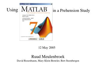
This report presents findings from an experimental study on hand shaping during grasping movements, focusing on the relationship between object size and the maximum aperture of the hand. Conducted by Ruud Meulenbroek and colleagues, the study involved 10 participants grasping cylinders of varying sizes under different visibility conditions. Data acquisition utilized Optotrak 3020 for precise motion tracking. Key performance variables were analyzed using MATLAB for preprocessing and statistical evaluation, underpinning the significance of visual and tactile information in grasping tasks.

Understanding Hand Shaping in Grasping: An Experimental Study on Object Size and Vision
E N D
Presentation Transcript
in a Prehension Study Using 12 May 2005 Ruud Meulenbroek David Rosenbaum, Mary Klein Breteler, Bert Steenbergen
Overview • Sneak Preview • Report of experimental results to colleagues • Use of Matlab • Principle • File I/O • Data preprocessing • Finding relevant time indices in behaviour • Plotting • Calculating critical performance variables • Time-normalizing functions • Creating a data matrix for statistical analyses • Write output file for SPSSX
Sneak preview- Report of experimental results to colleagues - Topic: “Hand shaping in grasping” • Background • Maximum aperture is linearly scaled to object size(Jeannerod 1981; Paulignan et al. 1991,1997; Smeets, 1999) • Research questions • Also when being blindfolded? • What about the rotations of the joints in the hand? Newell, K. M., Scully, D. M., McDonald, P. V., & Baillargeon, R. (1989). Task constraints and infant grip configurations. Developmental Psychobiology, 22, 817-832.
Sneak preview Theory • Motion planning • Entails goal-posture selection • Tuned to multiple task constraints Rosenbaum, D. A., Meulenbroek, R.G.J., Jansen, C., Vaughan, J. (2002). Posture-based motion planning: Applications to grasping. Psychological Review, 108, 708-734. Meulenbroek, R.G.J., Kappers, A.L., & Mutsaarts, M. (2001). Does haptic space play a role in the planning and execution of grasping movements? Poster presented at the 'Neural control of space coding and action production' meeting in Lyon (France), March 22-24, 2001
Sneak preview Simulation The orientation of the‘opposition axis’reflects the final arm-hand posture Fast movement Slow movement
Sneak preview Experiment • 10 Participants • 9 Objects (cylinders of appr. 20 cm height and a diameter of 0.3, 1.3, 2.3, 3.3, 4.3, 5.3, 6.3, 7.3, 8.3 cm) • 2 Modality Conditions: (Vision present versus absent; eyes open versus closed; ABBA counterbalancing) • 10 Replications (resulting in 180 trials per subject)
Sneak preview Experimental Task • The participant sat comfortably at a table... • with the left and right hand on two pieces of sandpaper fixated on the table top, appr. 20 cm in front of left and right shoulder • At the start of each trial the experimenter placed a cylinder in the non-dominant hand of the participant • The participant held the bottom half of the cylinder with opposing thumb and fingers (of the non-dominant hand) • An acoustic go-signal was presented • The participant’s task was to grasp with the dominant hand the top half of the cylinder that he/she held in the non-dominant hand • In half the trials the participant was asked to close his/her eyes before the cylinder was placed in his/her non-dominant hand
Optotrak 3020 (NDI, Canada) Upper arm Forearm “Rigid bodies” Infrared light emitting diodes Pen Trunk Hand Finger joints Infrared cameras Bouwhuisen, C.F., Meulenbroek, R.G.J., & Thomassen, A.J.W.M. (2002). A 3D motion-tracking method in graphonomic research: Possible applications in future handwriting recognition studies. International Journal of Pattern Recognition, 35(5), 1039-1047. Sneak preview Method Data acquisition
Sneak preview Data acquisition + • Optotrak 3020; two time-locked camera systems • 8 IREDs on the joints of the hand • Sampling rate of 200 Hz • Recording interval of 3 s • Preprocessing: low-pass filtering (<8 Hz)
6 7 5 8 Aperture (‘opposition axis’ ) 1 4 2 3 Sneak preview IRED configuration and aperture index
Use of Matlab Principle KISS : Keep It Simple Stupid (David Rosenbaum)
Use of Matlab Constants, loop parameters, toggle switches Give your matlab programme a sensible name! Clear entire memory! % segmentation.m % clear all; % constants Fs=200; % Hz sec=1/Fs; filtfreq_low=8; filtfreq_high=0.0; % number of subjects and data files ibsubject=1; iesubject=12; ibfile=1; iefile=180; % toggle switches iplot=1; filter=1; outputwanted=1; Set constants Set loop parameters Exploit toggle switches (0=Off;1=On)
Use of Matlab Windows, name of file with design codes % windows for plotting purposes if iplot==1 fig1=figure('position',[5 300 400 220]); fig2=figure('position',[400 300 400 220]); end; % subject loop for subject=ibsubject:iesubject, pp=subject % without semi-colon to provide feedback in command window! ppstr=int2str(pp); % read the data from the design file design.txt prefix=['C:\Ruud\Projects\Objectsize\data\pp' ppstr '\']; fname=['design']; ext=['.txt']; filename=[prefix fname ext]; eval(['load ' filename]); design=eval(fname);
Use of Matlab Design information, file loop, filename datafile % put design information in separate arrays trialnr=design(:,1); vision=design(:,2); cylinder_size=design(:,3); ntrials=length(trialnr); % data file loop for jfile=1:ntrials, % feedback on filenumber in command window file=trialnr(jfile) % again without semicolon! fstr=int2str(file); % pick up IRED displacement data ext=['.otd']; if jfile<10 fname=['C#000' fstr]; end; if jfile>9 & jfile<100 fname=['C#00' fstr]; end; if jfile>99 fname=['C#0' fstr]; end; filename=[prefix fname ext];
Use of MatlabRead data file fpread.m is separate m-file % read IRED displacement data from file [hdr,cdata] = fpfread(filename); X1 Y1 Z1 X2 Y2 Z2 Units: mm Time (samples)
% Detect missing data value (-36973140302885665500000000000.0000) % and interpolate linearly function [x]=interpolate_missing_data_points(s); mdv=-36973140302885665500000000000.0000; ns=length(s); if s(1)==mdv i=1; while s(i)==mdv i=i+1; end; s(1:i)=s(i+1); end; for i=2:ns-1, if s(i)==mdv ib=i-1; j=i; while ((s(j)==mdv) & (j<ns)) j=j+1; end; ie=j; if ie==ns if ib>1 for k=ib:ie, s(k)=s(ib-1); end; end end; ds=(s(ie)-s(ib))./(ie-ib+1); for k=ib:ie, s(k)=s(ib)+((k-ib+1).*ds); end; end; end; x=s; Use of MatlabPreprocessing IRED displacement data % interpolate missing data points ndim=size(cdata); ns_ireds=ndim(1); for idim=1:ndim(2), h=cdata(:,idim); hi=interpolate_missing_data_points(h); cdata(:,idim)=hi; end; % convert to cm for idim=1:ndim(2), cdata(:,idim)=cdata(:,idim)./10; end;
Use of MatlabPreprocessing IRED displacement data: A. filtering • Filter = 3rd-order Butterworth filter • Applied forward and backward to prevent phase shift % filter data for idim=1:ndim(2), h=cdata(:,idim); hf=filteren(h,Fs,filtfreq_low); cdata(:,idim)=hf; end; function[smooth]=filteren(data,Fs,Fc) % FILTEREN.M % function file voor filteren met verwijdering van de inslinger-effecten % Fs is de sample frequentie % Fc is de afsnijfrequentie [m,n]=size(data); Fs=Fs./2; [B,A]=butter(3,Fc/Fs); % 3e orde filter. % 6e orde low-pass filter, zero phase lag. for j=1:n smooth(:,j) = filtfilt(B,A,data(:,j)); end
Use of MatlabPreprocessing IRED displacement data: B. filtering • Filter = 3rd-order Butterworth filter • Applied forward and backward to prevent phase shift % filter data for idim=1:ndim(2), h=cdata(:,idim); hf=filteren(h,Fs,filtfreq_low); cdata(:,idim)=hf; end; Red = raw signal Blue = smoothed signal
Use of MatlabAdditional arrays to prepare plotting % number of samples, time axis, y=0 axis ns=ndim(1); t=[1:ns].*sec; t=t'; y0=zeros(1,ns); y0=y0';
Use of MatlabPrepare plotting of top view of hand IRED positions % put IRED data in separate 3D matrix for i=1:ndim(1), for j=1:8, j1=j; k=(j1-1).*3+1; handx(i,j)=cdata(i,k); handy(i,j)=cdata(i,k+1); handz(i,j)=cdata(i,k+2); end; end; cdata 600x24 115200 double array handx 600x8 38400 double array handy 600x8 38400 double array handz 600x8 38400 double array
Start End Use of MatlabPlot top view of hand % Plot XY plot if iplot==1, figure(fig1); set(gcf,'Color','white'); title('Top View'); hold on; axis equal; view(2); for i=1:4:600, plot3(handx(i,:),handy(i,:),handz(i,:),'k'); end; xlabel('X (cm)'); ylabel('Y (cm)'); end; % of if iplot==1
6 7 5 8 1 4 2 3 function [afgeleide]=afgeleid(data,sf) % AFGELEID.M % dit programma differentieert een willekeurige data set data die staat in een matrix % sf = samplefrequentie in Hz; Ron Jacobs, juli 1989 [m,n]=size(data); afgeleide=zeros(m,n); for i=3:m-2, afgeleide(i,:)=(-data(i-2,:)*1.5-data(i-1,:)*4+data(i+1,:)*4+data(i+2,:)*1.5)*(sf/14); end afgeleide(1,:) = afgeleide(3,:); afgeleide(2,:) = afgeleide(3,:); afgeleide(m,:) = afgeleide(m-2,:); afgeleide(m-1,:) = afgeleide(m-2,:); Use of MatlabDetermine wrist speed function % Determine wrist speed xw=handx(:,4); yw=handy(:,4); zw=handz(:,4); dxw=afgeleid(xw,Fs); dyw=afgeleid(yw,Fs); dzw=afgeleid(zw,Fs); vw=sqrt(dxw.^2+dyw.^2+dzw.^2);
Use of MatlabCheck wrist speed function % Check wrist speed function in command window plot(vw); xlabel(‘samples’); ylabel(‘wrist speed (cm/s);
Use of MatlabFind critical time indices in wrist speed function % Find start and end of movement and time index of maximum speed [vmax,tvmax]=max(vw); vthreshold=.05.*vmax; ib=tvmax; while vw(ib)>=vthreshold & ib>2 ib=ib-1; end; ie=tvmax; while vw(ie)>=vthreshold & ie<ns-1 ie=ie+1; end; ib ie tvmax threshold
6 7 5 8 1 4 2 3 Use of MatlabDetermine aperture-time function % Determine aperture-time function for i=1:ndim(1); dx=handx(i,1)-handx(i,8); dy=handy(i,1)-handy(i,8); dz=handy(i,1)-handy(i,8); aperture(i)=sqrt(dx.^2+dy.^2+dz.^2); end;
Use of MatlabCheck aperture-time function % Check aperture function in command window plot(aperture); xlabel(‘samples’); ylabel(‘aperture (cm);
Use of MatlabFind critical time indices in aperture-time function % Find maximum aperture and moment of maximum aperture [maxapt,tmaxapt]=max(aperture); mommaxapt=100.*((tmaxapt-ib)./(ie-ib)); maxapt tvmaxapt
Define reference lines of critical time indices for plotting % Data for reference line in plotting tref(1)=tmaxapt;tref(2)=tmaxapt; aptref(1)=0;aptref(2)=maxapt; % Data for reference line in plotting trefv(1)=tvmax;trefv(2)=tvmax; vwref(1)=0;vwref(2)=max(vws); Use of MatlabCalculate amplitude-scaled wrist speed function to plot simultaneously with aperture-time function % Calculate amplitude scaled wrist speed function scalefactor=max(aperture)./max(vw); vws=vw.*scalefactor;
Use of MatlabPlot aperture-time and normalized speed functions if iplot==1, figure(fig2); set(gcf,'Color','white'); title('Normalized Speed & Aperture')'; hold on; axis([t(ib) t(ie) 0 max(aperture)]); plot(t(ib:ie),aperture(ib:ie),'r'); plot(t(tref),aptref,'k'); plot(t(ib:ie),vws(ib:ie),'k-'); plot(t(trefv),vwref,'k'); xlabel('Time (s)'); ylabel('Aperture (cm)'); end; % of if iplot==1
Sneak preview Example: Prehension kinematics Normalized speed (arbitrary units) Aperture (cm) Time (s)
Sneak preview IRED configuration and joint angles 6 7 5 8 j5 j6 j4 1 j1 j3 j2 4 2 3
Use of MatlabDetermine joint angles in hand function[alfa]=angle2d_signed(pos1,pos2,pos3); % calculates the 2D joint angle % Mary Klein Breteler, March 2002 % orientation of first segment th=atan2(pos2(1)-pos1(1),pos2(2)-pos1(2)); % orientation of second segment relative to first segment Rz = [cos(th) -sin(th) 0; sin(th) cos(th) 0; 0 0 1]; vec = pos2(1:2) - pos3(1:2); vec = [vec/norm(vec) 0]; vecrot = (Rz*vec')'; % angle alfa=atan2(vecrot(1),vecrot(2)); beta=unwrap(alfa); alfa=beta.*180/pi; % only positive values if alfa < 0, alfa = alfa + 360; end % Constants degtorad=pi./180; radtodeg=1./degtorad; % Determine enclosed angle of hand joints (n=6) for ired=1:6, for i=1:ns, pos1(1)=handx(i,ired); pos1(2)=handy(i,ired); pos1(3)=handz(i,ired); pos2(1)=handx(i,ired+1); pos2(2)=handy(i,ired+1); pos2(3)=handz(i,ired+1); pos3(1)=handx(i,ired+2); pos3(2)=handy(i,ired+2); pos3(3)=handz(i,ired+2); joint(i,ired)=angle2d_signed(pos1,pos2,pos3); end; end;
j5 j6 j4 j1 j2 j3 Sneak preview Example: Joint rotations Note that joint angles may exceed 180 degs, partially due to their placement,i.e. imperfect alignment, and partially due to overextension.
Use of MatlabCalculating critical performance variables, e.g. % Find start and end of movement ib=fileib(jfile); ie=fileie(jfile); [vmax,tvmax]=max(vw(ib:ie)); tvmax=tvmax+ib; momvmax=100.*((tvmax-ib)./(ie-ib)); % Determine maximum and moment of maximum joint angles for j=1:6, [jointmax,tjointmax]=max(joint(ib:ie,j)); maxjntang(j)=jointmax; tmaxjntang(j)=100.*((tjointmax)./(ie-ib)); end;
Use of MatlabTime normalizing functions • Resample function to 50 data points • Write resampled function to output file • Process resampled functions in Excel/SPSSX % store time-normalized kinematic functions n1=ie-ib+1; n2=50; vwtn=time_normalize(vw(ib:ie),n1,n2); % function [tx]=time_normalize(x,n1,n2); % % x = 1-dimensionaal input array (check op rij of kolom array) % n1 = lengte van input array x % n2 = gewenste lengte van outputarray tx % function [tx]=time_normalize(x,n1,n2); s=1:n1; step=(n1-1)./(n2-1); si=1:step:n1; tx=interp1(s,x,si,'spline');
Use of MatlabCreating a data matrix for statistical analysis % clear output arrays output=zeros(15,1); if outputwanted==1 output(1)=pp; output(2)=file; output(3)=vision(file); % vision output(4)=objectsize(file); % size output(5)=(ie-ib).*sec; % MT output(6)=vmax; % peak speed output(7)=momvmax; % moment peak speed (%MT) output(8)=maxapt; % peak aperture (cm) …Etc.
Use of Matlab - Write outputfile for SPSSX % Write outputfile of, say 8 variables (independent + dependent) per observation if outputwanted==1 ext_out=['.dat']; fnameout=['output_new']; outname=[prefix fnameout ext_out]; fid=fopen(outname,'a'); f='%8.3f '; f_last='%8.3f\n'; % Take care number of f's equals number of output variables minus 1 outputformat=([f f f f f f f f_last]); fprintf(fid,outputformat,output); fclose(fid); end; % of outputwanted==1