Consumer Choice and Elasticity
350 likes | 518 Vues
Consumer Choice and Elasticity. 5. 20. 3. 7. Fundamentals of Consumer Choice. Law of diminishing marginal utility :. As the rate of consumption increases, the marginal utility derived from consuming additional units of a good will decline. Fundamentals of Consumer Choice.

Consumer Choice and Elasticity
E N D
Presentation Transcript
Consumer Choice and Elasticity 5 20 3 7
Fundamentals of Consumer Choice
Law of diminishing marginal utility: • As the rate of consumption increases, the • marginal utility derived from consuming • additional units of a good will decline. Fundamentals of Consumer Choice • Factors affecting choice: • Limited income necessitates choice. • Consumers make choices purposefully. • One good can be substituted for another. • Consumers must make decisions without perfect information, but knowledge and past experience will help.
Marginal Utility, Consumer Choice, and the Demand Curve of an Individual
The Demand Curve • The height of an individual's demand curve indicates the maximum price the consumer would be willing to pay for that unit. • A consumer's willingness to pay for a unit of a good is directly related to the utility derived from consumption of the unit. • The law of diminishing marginal utilityimplies that a consumer's marginal benefit, and thus the height of their demand curve, falls with the rate of consumption.
Jones’s demand curvefor frozen pizza MB1 MB2 MB3 Price = $2.50 MB4 d = MB < < < MB4 MB3 MB2 MB1 because < < < MU4 MU3 MU2 MU1 The Demand Curve • An individual’s demand curve, Jones’s demand for frozen pizzas in this case, reflects the law of diminishing marginal utility. Price $3.50 • Because marginal utility (MU) falls with increased consumption, so does a consumer’s maximum willingness to pay -- marginal benefit (MB). $3.00 $2.50 • A consumer will purchase until MB =Price. . . $2.00 so at $2.50 Jones would purchase 3 frozen pizzas and receive a consumer surplus shown by the shaded area (above the price line and below the demand curve). Frozen pizzasper week 1 2 4 3
MUb MUn MUa Pb Pn Pa Consumer Equilibrium With Many Goods • Each consumer will maximize his/her satisfaction by ensuring that the last dollar spent on each commodity yields an equal degree of marginal utility. = = . . . =
Price Changes and Consumer Choice • The demand curve shows the amount of a product consumers would be willing to buyat different prices for a specific period. • The law of demand states that there is an inverse relationship between the quantity of a product purchased and its price. • Reasons the demand curve slopes downward: • Substitution effect: as a product’s price falls, the consumer will buy more of it and less of other, now more expensive, products. • Income effect: as a product’s price falls, a consumer’s real income rises and so induces the individual to buy more of both it and other goods.
Time Cost and Consumer Choice • The monetary price of a good is not always a complete measure of its cost to the consumer. • Consumption of most goods requires time as well as money. Like money, time is scarce to the consumer. • So, a lower time cost, like a lower money price, will make a product more attractive. • Time costs, unlike money prices, differ among individuals.
1. Chuck is currently purchasing 3 pairs of jeans and 5 t-shirts per year. The price of jeans is $30, and t-shirts cost $10. At his current rate of consumption, his marginal utility of jeans is 60 and his marginal utility of t-shirts is 30. Is Chuck maximizing his utility? Would you suggest he buy more jeans and fewer t-shirts, or more t-shirts and fewer jeans? 2. “If the price of gasoline goes up and Fran now buys fewer candy bars because she has to spend more on gas, this would best be explained by the substitution effect.” -- Is this statement true or false? Questions for Thought:
Market Demand Reflects the Demand of Individual Consumers
D d d Individual and Market Demand Curves • Consider Jones’s demand for frozen pizza. At $3.50 Jonesdemands 1 pizza … at $2.50 3 pizzas … and so on … • Consider Smith’s demand for frozen pizza. At $3.50 Smithdemands 2 pizzas … at $2.50 3 pizzas … and so on … • The market demand curveis merely the horizontal sum of the individual demand curves (here Jones and Smith). • The market demand curvewill slope downward to the right, just as the individual demand curves do. Jones Smith 2-Person market Price Price Price $3.50 $3.50 $3.50 $2.50 $2.50 $2.50 1 2 3 4 5 6 7 8 1 2 3 4 5 6 7 8 1 2 3 4 5 6 7 8 Weekly frozen pizza consumption
Price Elasticityof demand = = % Change in quantity demanded % Q = % P % Change in Price - + ( Q Q ) ( Q Q ) 0 1 0 1 = - + ( P P ) ( P P ) 0 1 0 1 Price Elasticity of Demand • Price elasticity reveals the responsiveness of the amount purchased to a change in price. - or put more simply -
= -2.17 = - Recall - Price Elasticityof demand = % Q -33.33 15.38 % P Price Elasticity Numerical Application • Suppose Trina bakes specialty cakes. She can sell 50 specialty cakes per week at $7 a cake, or 70 specialty cakes per week at $6 a cake. • What is the demand elasticity for Trina’s cakes? Percent change in quantity demanded: Percent change in price: The price elasticity of demand equals:
Price Elasticity of Demand • After calculating the price elasticity of demand, you can determine whether it is elastic, inelastic, or unitary elastic with the following: • If the absolute value of the elasticity term < 1,then the demand is inelastic. • If the absolute value of the elasticity term > 1,then the demand is elastic. • If the absolute value of the elasticity term = 1,then the demand is unitary elastic. • Because price elasticity of demand is always negative, the sign on the coefficient is often omitted in discussions of elasticity.
Price • Perfectly inelastic:An increase in price results in no change in consumers purchases. The vertical demand curve is mythical as the substitution and income effects prevent this from happening in the real world. Mythicaldemandcurve Quantity/time (a) Price • Relatively inelastic: A percent increase in price results in a smaller % reduction in sales. The demand for cigarettes has been estimated to be highly inelastic. Demand for Cigarettes Quantity/time (b) Elasticity of Demand
Price • Unitary elasticity:The percent change in quantity demanded due to an increase in price is equal to the % change in price. A decreasing slope results. Sales revenue (price times quantity) is constant. Demand curve of unitary elasticity Quantity/time (c) Elasticity of Demand
Relatively elastic:A % increase in price leads to a larger % reduction in purchases. When there are good substitutes for a product (as with Granny Smith apples), the quantity purchased will be highly sensitive to changes in price. Price Demand for Granny Smith apples Quantity/time (d) Price • Perfectly elastic: Consumers will buy all of Farmer Jones’s wheat at the market price, but none will be sold above the market price. Demand for Farmer Jones’s wheat Quantity/time (e) Elasticity of Demand
Recall - (110 - 100) (110 + 100) ($1 - $2) ($1 + $2) = Elasticity (-) 0.14 Elasticity of Demand Price • With this straight-line (constant-slope) demand curve, demand varies across a range of prices. = ( - ) 0.14 • Using the equation for elasticity, the formula shows that, when price rises • from $1 to $2 … while quantity demanded falls from 110 to 100 … the elasticity for that region of the demand curve is ( - 0.14 ) – inelastic. 2 1 D Quantity demanded 100 110
Recall - (20 - 10) (20 + 10) ($10 - $11) ($10 + $11) = Elasticity (-) 7. 0 Elasticity of Demand Price • A price increase of the same amount, from $10 to $11, . . . leads to a decline in quantity demanded from 20 to 10. = (-) 7.0 11 10 • Note that this change in price was smaller (as a %) than in the previous slide but resulted in the same change in quantity demanded. • Applying the elasticity formula, the calculated elasticity is (- 7.0) – greater than (- 0.14) from before. • The price-elasticity of a straight-line demand curve increases as price rises. D Quantity demanded 10 20
Determinants of Price Elasticity of Demand • Availability of substitutes • When good substitutes for a product are available, a rise in price induces many consumers to switch to another product. • The greater the availability of substitutes, the more elastic demand will be. • Share of total budget expended on product • As the share of the total budget spent on the product increases, demand is more elastic.
Elastic and Inelastic Demand Price Price $6.00 $6.00 $4.00 $4.00 D D 100 25 90 100 (a) 1/2 lb. hamburgers per week (in thousands) (b) Cigarette packs per week (in millions) • As the price of 1/2 lb. hamburgers (a) rises from $4.00 to $6.00 ... the quantity demanded plunges from 100,000 to 25,000 per week. • The % reduction in quantity demanded is larger than the % increase in price, hence the demand for 1/2 lb hamburgers is relatively elastic. • As the price of cigarettes (b) rises from $4.00 to $6.00 . . . quantity demanded declines from 100 million to 90 million packs per week. • The % reduction in quantity demanded is smaller than the % increase in price, hence the demandfor cigarettes is relatively inelastic.
Time and Demand Elasticity • If the price of a product increases, consumers will reduce their consumption by a larger amount in the long run than in the short run. • Thus, demand for most products will be more elastic in the long run than in the short run. • This relationship is sometimes referred to as the second law of demand.
Inelastic Approximately Unitary Elasticity Movies - 0.9 Salt - 0.1 Homes, owner occupied (long run) - 1.2 Matches - 0.1 Shellfish (consumed at home) - 0.9 Toothpicks - 0.1 Oysters (consumed at home) - 1.1 Airline travel (short run) - 0.1 Private education - 1.1 Gasoline (short run) - 0.2 Tires (short run) - 0.9 Gasoline (long run) - 0.7 Tires (long run) - 1.2 Natural gas, home (short run) - 0.1 Radio and television receivers - 1.2 Natural gas, home (long run) - 0.5 Coffee - 0.3 Fish (cod), at home - 0.5 Elastic Tobacco products (short run) - 0.5 Legal services (short run) - 0.4 Restaurant meals - 2.3 Physician services - 0.6 Foreign travel (long run) - 4.0 Taxi (short run) - 0.6 Airline travel (long run) - 2.4 Automobiles (long run) - 0.2 Fresh green peas - 2.8 Automobiles (short run) - 1.2 to -1.5 Chevrolet automobiles - 4.0 Fresh tomatoes - 4.6 Elasticity of Demand • Can you explain why the demand for some goods is highly inelastic while that for others is elastic.
How Demand Elasticity and Price Changes Affect Total Expenditures (or Revenues)on a Product
1 to decrease increase -- unchanged -- unchanged -- -- increase decrease Total Expenditures and Demand Elasticity Impact of higher priceon total consumer expenditures or a firm’s total revenue Impact of lower priceon total consumerexpenditures or a firm’s total revenue Elasticitycoefficient(in absolute value) Price elasticityof demand Elastic Unitary Elastic 1 Inelastic 0 to 1 • The table above summarizes the relationship between changes in price and total expenditures for demand curves of varying elasticity.
Income Elasticityof demand = % Change in quantity demanded % Change in Income Income Elasticity • Income elasticityindicates the responsiveness of a product’s demand to a change in income. • Anormal goodis a good with a positive income elasticity of demand. • As income expands, the demand for normal goods will rise. • Goods with a negative income elasticity are called inferior goods. • As income expands, the demand for inferior goods will decline.
Low Income Elasticity High Income Elasticity Margarine - 0.20 Private education 2.46 Fuel 0.38 New Cars 2.45 Electricity 0.20 Recreation and amusements 1.57 Fish (haddock) 0.46 Alcohol 1.54 Food 0.51 Tobacco 0.64 Hospital care 0.69 Income Elasticity of Demand • Why is the income elasticity of demand for some goods greater than for others? • What does it mean that the income elasticity of demand for margarine is negative? Can you think of any other goods which you would expect to have a negative income elasticity of demand coefficient?
Price Elasticity of Supply • The price elasticity of supplyis the percent change in quantity supplied divided by the percent change of the price causing the supply response. • analogous to the price elasticity of demand • If the % change in quantity is small relative to the % change in price, supply is inelastic. • If the % change in quantity is large relative to the % change in price, supply is elastic. • However, price elasticity of supply is positive because the quantity producers are willing to supply is directly related to price.
1. (a) Studies indicate that the demand for Florida oranges, Bayer aspirin, watermelons, and airfares to Europe are elastic. Why? (b) Why is the demand for salt, matches, and gasoline (short-run) inelastic? • 2. Are the following statements true or false? Explain your answers. • (a) A 10% reduction in price that leads to a 15% increase in amount purchased indicates a price elasticity of more than 1. (b) A 10% reduction in price that leads to a 2% increase in total expenditures indicates a price elasticity of more than 1. Questions for Thought:
3. Suppose Bobby, the owner-manager of Bobby’s Red Hot BBQ restaurant, projects the following demand for his baby-back rib platter: Price Quantity purchased ---------------------------------------------- $9 110 per night $11 100 per night $13 80 per night (a) Calculate the price elasticity of demand between $9 and $11. Was demand in this price range elastic, inelastic, or unitary? (b) Calculate the price elasticity between $11 and $13. Is it elastic, inelastic, or unitary? Questions for Thought: