Gene Mapping: Linkage and Association Analysis for Disease Identification
420 likes | 456 Vues
Learn about the two main approaches in gene mapping - linkage and association analyses - and how they help in identifying disease-causing genes in this comprehensive guide.

Gene Mapping: Linkage and Association Analysis for Disease Identification
E N D
Presentation Transcript
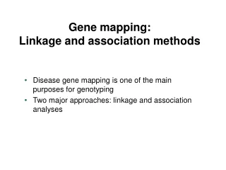
Disease gene mapping is one of the main purposes for genotyping Two major approaches: linkage and association analyses Gene mapping:Linkage and association methods
Try to localize genes affecting specific phenotypes Search for: co-segregation of disease and marker alleles Linkage analysis
Idea of Linkage Analysis Types of Linkage Analysis Parametric Linkage Analysis Conclusions Basics of Linkage Analysis
Idea of Linkage Analysis Types of Linkage Analysis Parametric Linkage Analysis Conclusions Basics of Linkage Analysis
One of the two main approaches in gene mapping. Uses pedigree data. Linkage Analysis
Two loci are linked if they appear nearby in the same chromosome. The task of linkage analysis is to find markers that are linked to the hypothetical disease locus Complex diseases in focus usually need to search for one gene at a time Requires mathematical modelling of meiosis Genetic linkage and linkage analysis
Number of crossover sites is thought to follow Poisson distribution. Their locations are generally random and independent of each other. Meiosis and crossover
DIS Marker The simple idea • Recombination fraction Always: 0 ≤ ≤ 0.5 • Task: Find that maximises L( |data ) • Obtain measure for degree of evidence in favour of linkage (LOD score)
Polymorphic loci whose locations are known Most often SNPs or microsatellites Inherited within the chromosomes 1 2 4 3 2 1 3 4 2 3 1 2 Father Mother 2 3 1 4 3 1 Child Markers and inheritance
Two individuals share same allele label they share the allele IBS (identical by state) Two individuals share an allele with same (grand)parental origin they share an allele IBD (identical by descent) IBS sharing can easily be deduced from genotypes. IBD sharing requires more information. One can try to deduce IBD sharing based on family structure and inheritance. Markers and information
Markers and information 1,2 2,3 The children share allele 1 IBS. They also share it IBD. 1,2 1,3
Markers and information 1,2 1,3 The children share allele 1 IBS. 1,2 1,3 They do not share alleles IBD.
Markers and information 1,1 2,3 The children share allele 1 IBS. 1,2 1,3 They either share or do not share it IBD.
Chr. 1 1 2 1 12 1 2 1 1 2 1 1 5 2 14 1 3 2 1 2 2 Chr. 2 1 3 4 5 1 2 3 2 4 2 1 3 4 4 7 1 4 3 4 4 2 3 Chr. 22 2 1 1 3 2 2 2 3 3 4 Building blocks of linkage analysis Marker maps Pedigree structures Genotypes Phenotypes
Information about disease model (in parametric analysis) Building blocks of linkage analysis (aa), probability of a homozygote being affected (Aa), probability of a heterozygote being affected (AA), probability of a non-carrier being affected (phenocopy rate) • Assumed disease allele frequency • Marker allele frequencies • Information about environmental variables
Idea of Linkage Analysis Types of Linkage Analysis Parametric Linkage Analysis Conclusions Basics of Linkage Analysis
Parametric vs. non-parametric Dichotomous vs. continuous phenotypes Elston-Stewart vs. Lander-Green vs. heuristic Two-point vs. multipoint Genome scan vs. candidate gene Types of linkage analysis
Idea of Linkage Analysis Types of Linkage Analysis Parametric Linkage Analysis Conclusions Basics of Linkage Analysis
A common approach in statistical estimation Define hypotheses Generate likelihood function Estimate Test hypotheses Draw statistical conclusions Maximum likelihood estimation
H0: = 0.5 the disease locus isnot linked to the marker(s) HA: 0.5 the disease locus is linked to the marker(s) Hypotheses in linkage analysis
Lj = gF P(gF) P(yF | gF)gM P(gM)P(yM | gM)gOi P(gOi | gF, gM) P(yOi | gO) The parameter is incorporated here Likelihood function for a single nuclear family G = genotype probabilitiesy = phenotype probabilities
The likelihood functions of multiple independent families are combined: L = Lj or logL = log Lj Several independent families
Compute values of likelihood function under null and alternative hypotheses. Their relationship is expressed by LOD score (essentially derived from the likelihood ratio test statistic. Testing of hypotheses
P-value gives a probability that a null hypothesis is rejected even though it was true. A LOD-score threshold of 3 corresponds to a single-test p-value of approximately 0.0001 Often, the significant areas pointed out are quite large, from 10-40 cM (millions of basepairs) On significance levels
0.56 0.5 LOD score 0.0 0.0 0.14 0.5 Recombination fraction LOD>3 taken as evidence of linkage.
Idea of Linkage Analysis Types of Linkage Analysis Parametric Linkage Analysis Conclusions Basics of Linkage Analysis
Linkage analysis is a pedigree-based approach to gene mapping. Parametric vs. nonparametric methods. Hypothesis-driven vs. explorative analysis. Meta-analysis (integration of several studies into “one big study”) becoming increasingly popular. Conclusions
After successful linkage analysis, what to do? How to refine the linked area – where actually the disease susceptibility locus is? Outline of the rest of the lecture: Allelic association χ2 –test LD mapping Fine mapping and association analysis
An example: A leukaemia study, where a number of affected and healthy control persons have been contacted for DNA samples A candidate gene has been suggested: GSTM1, which functions in the metabolism of benzene GSTM1 has two different alleles, 1 and 2, where A person is “positive” for allele 1 if his genotype is 1 1 or 1 2 A person is “null”, if having genotype 2 2 The numbers of leukaemic and control individuals either positive or null with respect to allele 1 are compared by χ2-test in order to find out, whether there is statistically significant difference Allelic association
Results: observed frequencies Expected frequencies Allelic assosiation
The observed are compared to expected frequencies. (null hypothesis, H0: carrier status and disease occurrence are independent of each other ) Test statistic where oi is the observed frequency for class i, ei the expected frequency for class i k is the number of classes Test statistic
Now, χ2 = 111,39. Degrees of freedom for the test: df=(r-1)(s-1), where r = number of rows, s = number of columns Here, df = (2-1)*(2-1) = 1 The χ2 value is then compared to the null distribution of critical χ2-test statistic values (within the given df class) Allelic assosiation
df\p 0.10 .05 .025 .01 .005 1 2.71 3.84 5.02 6.63 7.88 2 4.61 5.99 7.38 9.21 10.60 3 6.25 7.81 9.35 11.34 12.84 4 7.78 9.49 11.14 13.28 14.86 5 9.24 11.07 12.83 15.09 16.75 6 10.64 12.59 14.45 16.81 18.55 7 12.02 14.07 16.01 18.48 20.28 8 13.36 15.51 17.53 20.09 21.96 9 14.68 16.92 19.02 21.67 23.59 10 15.99 18.31 20.48 23.21 25.19 11 17.28 19.68 21.92 24.73 26.76 χ2-distribution: critical values for chosen significance levels When the observed value of test statistic is greater than the critical value (for the chosen significance levels) given in the table, the null hypothesis can be rejected.
The value we obtained, χ2 = 111,39 , exceeds all critical values with df=1 given in the table. We conclude, that H0 can be rejected and thus, there is statistically significant difference between the affected and healthy with respect to GSTM1 genotypes. The relative frequencies of ’null’ and ’positive’ genotypes show the same It seems that different GSTM1 genotypes, by changing the benzene metabolism, considerably affect the probability of getting leukaemia Allelic association
Note: compared to linkage analysis, which is based on the observed inheritance patterns in pedigrees, the association analysis studies correlation of allele presence and a disease in the level of population We find an allele or a haplotype overrepresented in affected individuals → BUT the statistical correlation does not implicate a causal relationship !!!! → Quite often, the associating allele or haplotype is not the cause of the disease itself, but is merely correlated with the presence of the actual susceptibility gene in the same chromosome. It is then said to be in linkage disequilibrium with the disease gene. →
6 2 1 3 1 2 5 3 Original mutation in one chromosome in the founder population A Time Current generation C B An affected pedigree
The marker itself is NOT the reason for the disease, but it’s located nearby the disease susceptibility gene, and there is correlation between the presence of certain marker allele and the disease gene allele (LD) The correlation, i.e. LD, is based on founder effect: the disease allele has been born a long time ago on a certain ancestral chromosome, and majority of disease alleles existing presently predate from that original mutation LD mapping
Data Disease locus Disease status SNP1 S2 ... ... a ? 2 1 1 a ? 1 2 1 1 2 2 1 1 2 1 2 1 2 1 1 2 2 1 2 2 1 2 1 1 2 2 1 1 1 1 1 1 1 c 2 1 ? ?c 1 1 ? ? 1 2 2 1 1 2 1 1 2 2 2 1 1 1 a 1 1 2 1a 1 1 1 2 1 1 2 1 1 2 2 2 2 2 1 1 2 1 2 2 ? 1 1 1 ? 1 … … … …
”old-fashioned” allele association with some simple test (problem: multiple testing) TDT; modelling of LD process: Bayesian, EM algorithm, integrated linkage & LD Many approaches, several programs
The amount of LD is on a continuous but slow change, where the natural forces of genetic drift population structure natural selection new mutations founder effect ...affect it – even if two pairs of loci are in exactly the same distance from each other, their amount of LD may vary a lot. → This limits the accuracy of LD mapping, though it is much more accurate in pinpointing the location of a disease gene compared to linkage Limitations: LD is random process