Influence Maximization in Continuous Time Diffusion Networks
Manuel Gomez Rodriguez Bernhard Schölkopf. Influence Maximization in Continuous Time Diffusion Networks. 29.06.12, ICML ‘12. Propagation. Propagation takes place on. We can extract propagation traces from. Information Networks. Social Networks. Recommendation Networks. Epidemiology.

Influence Maximization in Continuous Time Diffusion Networks
E N D
Presentation Transcript
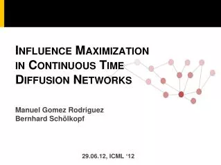
Manuel Gomez RodriguezBernhard Schölkopf Influence Maximizationin Continuous TimeDiffusion Networks • 29.06.12, ICML ‘12
Propagation • Propagation takes place on • We can extract propagation traces from • Information Networks • Social Networks • Recommendation Networks • Epidemiology • Human Travels
Influence Maximization T 0 • Our aim: Find the optimal source nodes that maximize the average number of infected nodes by T: T 0
Continuous time vs sequential model • TRADITIONALLY… j i Probability of transmission • Propagation has been modeled as sequential rounds in discrete time steps #greeceretweets • HOWEVER, REAL TIME MATTERS… • IN OUR WORK… j i Likelihood of transmission • Propagation ismodeled as a continuous process with different rates
Influence Maximization: Outline Describe the evolution of a diffusion process mathematically Analytically compute the influence in continuous time Efficiently find the source nodes that maximizes influence Validate InfluMax on synthetic and real diffusion data
Sources and sink node n • Set of source nodes A: Nodes in which a diffusion process starts • Sink node n: Node under study. We aim to evaluate its probability of infection before T given A: P(tn < T | A) Source node Sink node n
Given asink noden and a set of infected nodesI, we define thedisabled nodesSn(I) dominated by I: Domination: disabled nodes • A node u is disabled if any path from u to n visits at least one infected node 2 9 n 1 Infected node 4 3 Sink node n 8 5 Disabled node 6 7 6 7
Self domination: disabled sets We define the set of self-dominant disabled sets : Nodes in a self-dominant disable set only block themselves relative to the sink node n Infected Sink node n 2 1 9 8 4 3 5 6 7 We can find them all efficiently!
Monitoring a diffusion process • Given asink noden and a diffusion process starting in asource set A: We show that a diffusion process can be described by the state space of self-dominant disabled sets This means that… The probability of infecting the sink node n before T is the probability of reaching a specific disabled set before T
Diffusion process: continuous time • Given a diffusion process, how fast do we traverse from one self-dominant disable set to another? Disabled set III Disabled set I Disabled set IV Disabled set II j i It depends on how quickly information propagates between each pair of nodes Likelihood of transmission
Diffusion process as a CTMC Theorem. Given a source set A, a sink node n and independent exponential likelihoods , the process is a CTMC with state space This means that… The probability of infection of the sink node n before T is a phase type distribution Exp matrix depends on and T
Computing influence We sum up over all nodes in the network We know how to compute the probability of infection of any sink node n before T INFLUENCE
Maximizing the influence Until now, we show how to compute influence. However, our aim is to find the optimal set of sources nodes A that maximizes influence: (1) • Unfortunately, Theorem. The continuous time influence maximization problem defined by Eq. (1) is NP-hard.
Submodular maximization There is hope! The influence function satisfies a natural diminishing property: Theorem. The influence function is a submodular function in the set of nodes A. • We can efficiently obtain a suboptimal solution with a 63% provable guarantee • using a greedy algorithm
Experimental Setup We validate our method on: Synthetic data 1. Generate network structure 2. Assign transmission rate to each edge in the network 3. Run InfluMax Real data 1. MemeTracker data (172m news articles 08/2009– 09-2009) 2. We infer diffusion networks from hyperlink or memes cascades 3. Run InfluMax • What is the optimal source set that maximizes influence? • How does the optimal source set change with T? • How fast is the algorithm?
Influence vs. number of sources 1024-node Hierarchical Kronecker 512-node Random Kronecker 1024-node Forest Fire • Performance does not depend on the network structure: • Synthetic Networks: Forest Fire, Kronecker, etc. • InfluMax typically outputs source sets that results in a 20% higher influence than competitive methods!
Influence vs. time horizon T = 0.1 The source set outputted by InfluMax can change dramatically with the time horizon T For which time horizon does InfluMax gives the greatest competitive advantage? T = 1
Influence vs. time horizon 1024-node Hierarchical Kronecker network • In comparison with other methods, InfluMax performs best for relatively small time horizon.
Real data: Influence vs. # of sources 1000-node real network (inferred from MemeTracker cascades) 1000-node real network (inferred from hyperlink cascades) • InfluMax outputs a source set that results in a 20-25% higher influence than competitive methods!
Conclusions We model diffusion and propagation processes in continuous time: We make minimal assumptions about the physical, biological or cognitive mechanisms responsible for diffusion. The model uses only the temporal traces left by diffusion. • Including continuous temporal dynamics allows us to evaluate influence analytically using CTMCs. • Once we compute the CTMC, it is straight forward to evaluate how changes in transmission rates impact influence • Natural follow-up: use event history analysis/hazard analysis to generalize our model
Thanks! Code & More: http://www.stanford.edu/~manuelgr/influmax/

