Statistics and ANOVA
Statistics and ANOVA. ME 470 Fall 2013. Here are some interesting on-the-spot designs from the past and this class. Winner, Spring 2010 15” Tall 8$ Cost 0.533 Cost/Height. Fall 2009, 0.27 Cost/Height. Fall 2011 Height = 12 Cost = 6 Cost/Height = 0.5. Fall 2011 Height = 24 Cost = 12

Statistics and ANOVA
E N D
Presentation Transcript
Statistics and ANOVA ME 470 Fall 2013
Here are some interesting on-the-spot designs from the past and this class. Winner, Spring 2010 15” Tall 8$ Cost 0.533 Cost/Height Fall 2009, 0.27 Cost/Height
Fall 2011 Height = 12 Cost = 6 Cost/Height = 0.5 Fall 2011 Height = 24 Cost = 12 Cost/height = 0.5
I really enjoy the on-the-spot design. • What did you learn about the design process? • There are many challenges in product development • Trade-offs • Dynamics • Details • Time pressure • Economics • Why do I love product development? • Getting something to work • Satisfying societal needs • Team diversity • Team spirit Design is a process that requires making decisions.
Product Development Phases Concept Development System-Level Design Detail Design Testing and Refinement Production Ramp-Up Planning Concept Development Process You will practice the entire concept development process with your group project Mission Statement Development Plan Identify Customer Needs Establish Target Specifications Generate Product Concepts Select Product Concept(s) Test Product Concept(s) Set Final Specifications Plan Downstream Development Perform Economic Analysis Benchmark Competitive Products Build and Test Models and Prototypes
We will use statistics to make good design decisions! We will categorize populations by the mean, standard deviation, and use control charts to determine if a process is in control. We may be forced to run experiments to characterize our system. We will use valid statistical tools such as Linear Regression, DOE, and Robust Design methods to help us make those characterizations.
Cummins asked a capstone group to investigate improvements for turbo charger lubrication sealing. 5.9L High Output Cummins Engine
Cummins Inc. was dissatisfied with the integrity of their turbocharger oil sealing capabilities.
Here are pictures of oil leakage. Oil Leakage into Compressor Housing Oil Leakage on Impellor Plate The students developed four prototypes for testing. After testing, they wanted to know which solution to present to Cummins. You will analyze their data to make a suggestion.
How can we use statistics to make sense of data that we are getting? • Quiz for the day • What can we say about our M&Ms? • We will look at the results first and then you can do the analysis on your own.
Statistics can help us examine the data and draw justified conclusions. • What does the data look like? • What is the mean, the standard deviation? • What are the extreme points? • Is the data normal? • Is there a difference between years? Did one class get more M&Ms than another? • If you were packaging the M&Ms, are you doing a good job? • If you are the designer, what factors might cause the variation?
If I am a plant manager, do I like one distribution better than another?
How do we interpret the boxplot? largest value excluding outliers B o x p l o t o f B S N O x Q3 2 . 4 5 2 . 4 0 (Q2), median 2 . 3 5 x O N S B 2 . 3 0 Q1 2 . 2 5 2 . 2 0 outliers are marked as ‘*’ smallest value excluding outliers Values between 1.5 and 3 times away from the middle 50% of the data are outliers.
The Anderson-Darling normality test is used to determine if data follow a normal distribution. If the p-value is lower than the pre-determined level of significance, the data do not follow a normal distribution.
Anderson-Darling Normality Test Measures the area between the fitted line (based on chosen distribution) and the nonparametric step function (based on the plot points). The statistic is a squared distance that is weighted more heavily in the tails of the distribution. Anderson-Smaller Anderson-Darling values indicates that the distribution fits the data better. The Anderson-Darling Normality test is defined as: H0: The data follow a normal distribution. Ha: The data do not follow a normal distribution. Another quantitative measure for reporting the result of the normality test is the p-value. A small p-value is an indication that the null hypothesis is false. (Remember: If p is low, H0 must go.) P-values are often used in hypothesis tests, where you either reject or fail to reject a null hypothesis. The p-value represents the probability of making a Type I error, which is rejecting the null hypothesis when it is true. The smaller the p-value, the smaller is the probability that you would be making a mistake by rejecting the null hypothesis. It is customary to call the test statistic (and the data) significant when the null hypothesis H0 is rejected, so we may think of the p-value as the smallest level α at which the data are significant.
You can use the “fat pencil” test in addition to the p-value. Note that our p value is quite low, which makes us consider rejecting the fact that the data are normal. However, in assessing the closeness of the points to the straight line, “imagine a fat pencil lying along the line. If all the points are covered by this imaginary pencil, a normal distribution adequately describes the data.” Montgomery, Design and Analysis of Experiments, 6th Edition, p. 39 If you are confused about whether or not to consider the data normal, it is always best if you can consult a statistician. The author has observed statisticians feeling quite happy with assuming very fat lines are normal. For more on Normality and the Fat Pencil http://www.statit.com/support/quality_practice_tips/normal_probability_plot_interpre.shtml
Walter Shewhart Developer of Control Charts in the late 1920’s You did Control Charts in DFM. There the emphasis was on tolerances. Here the emphasis is on determining if a process is in control. If the process is in control, we want to know the capability. www.york.ac.uk/.../ histstat/people/welcome.htm
What does the data tell us about our process? SPC is a continuous improvement tool which minimizes tampering or unnecessary adjustments (which increase variability) by distinguishing between special cause and common cause sources of variation Control Charts have two basic uses: Give evidence whether a process is operating in a state of statistical control and to highlight the presence of special causes of variation so that corrective action can take place. Maintain the state of statistical control by extending the statistical limits as a basis for real time decisions. If a process is in a state of statistical control, then capability studies my be undertaken. (But not before!! If a process is not in a state of statistical control, you must bring it under control.) SPC applies to design activities in that we use data from manufacturing to predict the capability of a manufacturing system. Knowing the capability of the manufacturing system plays a crucial role in selecting the concepts.
Voice of the Process Control limits are not spec limits. Control limits define the amount of fluctuation that a process with only common cause variation will have. Control limits are calculated from the process data. Any fluctuations within the limits are simply due to the common cause variation of the process. Anything outside of the limits would indicate a special cause (or change) in the process has occurred. Control limits are the voice of the process.
The capability index depends on the spec limit and the process standard deviation. Cp = (allowable range)/6s = (USL - LSL)/6s LSL USL (Upper Specification Limit) LCL UCL (Upper Control Limit) http://lorien.ncl.ac.uk/ming/spc/spc9.htm
Upper Control Limit for 2008 Lower Control Limit for 2008
Minitab prints results in the Session window that lists any failures. Test Results for I Chart of StackedTotals by C4 TEST 1. One point more than 3.00 standard deviations from center line. Test Failed at points: 129 TEST 2. 9 points in a row on same side of center line. Test Failed at points: 15, 110, 111, 112, 113 TEST 5. 2 out of 3 points more than 2 standard deviations from center line (on one side of CL). Test Failed at points: 52, 66, 119, 160, 161 TEST 6. 4 out of 5 points more than 1 standard deviation from center line (on one side of CL). Test Failed at points: 91, 97 TEST 7. 15 points within 1 standard deviation of center line (above and below CL). Test Failed at points: 193, 194, 195, 196, 197, 198, 199, 200
This chart is extremely helpful for deciding what statistical technique to use. X Data Multiple Xs Single X X Data X Data Discrete Continuous Discrete Continuous Discrete Logistic Regression Multiple Logistic Regression Multiple Logistic Regression Single Y Chi-Square Discrete Y Data Y Data Y Data Continuous One-sample t-test Two-sample t-test ANOVA Simple Linear Regression Multiple Linear Regression Continuous ANOVA Multiple Ys
When to use ANOVA • The use of ANOVA is appropriate when • Dependent variable is continuous • Independent variable is discrete, i.e. categorical • Independent variable has 2 or more levels under study • Interested in the mean value • There is one independent variable or more • We will first consider just one independent variable
ANOVA Analysis of Variance • Used to determine the effects of categorical independent variables on the average response of a continuous variable • Choices in MINITAB • One-way ANOVA • Use with one factor, varied over multiple levels • Two-way ANOVA • Use with two factors, varied over multiple levels • Balanced ANOVA • Use with two or more factors and equal sample sizes in each cell • General Linear Model • Use anytime!
Practical Applications • Determine if our break pedal sticks more than other companies • Compare 3 different suppliers of the same component • Compare 6 combustion recipes through simulation • Determine the variation in the crush force • Compare 3 distributions of M&M’s • And MANY more …
The null hypothesis for ANOVA is that there is no difference between years. General Linear Model: StackedTotals versus C4 Factor Type Levels Values C4 fixed 3 2008, 2010, 2011 Analysis of Variance for StackedTotals, using Adjusted SS for Tests Source DF Seq SS Adj SS Adj MS F P C4 2 6.6747 6.6747 3.3374 4.71 0.010 Error 203 143.8559 143.8559 0.7086 Total 205 150.5306 S = 0.841813 R-Sq = 4.43% R-Sq(adj) = 3.49% This p value indicates that the assumption that there is no difference between years is not correct!
The p value indicates that there is a difference between the years. The Tukey printout tells us which years are different. Grouping Information Using Tukey Method and 95.0% Confidence C4 N Mean Grouping 2010 57 7.9 A 2008 86 7.7 A B 2011 63 7.4 B Means that do not share a letter are significantly different. The averages for 2010 and 2008 are not statistically different. The averages for 2008 and 2011 are not statistically different.
Command:>Stat>Basic Statistics>Display Descriptive Statistics
If I am a plant manager, do I like one distribution better than another?
>Stat>Basic Statistics>Normality Test Select 2008
The Anderson-Darling normality test is used to determine if data follow a normal distribution. If the p-value is lower than the pre-determined level of significance, the data do not follow a normal distribution.
Command:>Stat>Control Charts>Variable Charts for Individuals>Individuals
When doing control charts for ME470, select all tests. It may be hard to see, but highlight the “tests” tab.
Minitab prints results in the Session window that lists any failures. Test Results for I Chart of StackedTotals by C4 TEST 1. One point more than 3.00 standard deviations from center line. Test Failed at points: 129 TEST 2. 9 points in a row on same side of center line. Test Failed at points: 15, 110, 111, 112, 113 TEST 5. 2 out of 3 points more than 2 standard deviations from center line (on one side of CL). Test Failed at points: 52, 66, 119, 160, 161 TEST 6. 4 out of 5 points more than 1 standard deviation from center line (on one side of CL). Test Failed at points: 91, 97 TEST 7. 15 points within 1 standard deviation of center line (above and below CL). Test Failed at points: 193, 194, 195, 196, 197, 198, 199, 200
Upper Control Limit for 2008 Lower Control Limit for 2008
Command: >Stat>ANOVA>General Linear Model
The null hypothesis for ANOVA is that there is no difference between years. General Linear Model: StackedTotals versus C4 Factor Type Levels Values C4 fixed 3 2008, 2010, 2011 Analysis of Variance for StackedTotals, using Adjusted SS for Tests Source DF Seq SS Adj SS Adj MS F P C4 2 6.6747 6.6747 3.3374 4.71 0.010 Error 203 143.8559 143.8559 0.7086 Total 205 150.5306 S = 0.841813 R-Sq = 4.43% R-Sq(adj) = 3.49% This p value indicates that the assumption that there is no difference between years is not correct!
Command: >Stat>ANOVA>General Linear Model
The p value indicates that there is a difference between the years. The Tukey printout tells us which years are different. Grouping Information Using Tukey Method and 95.0% Confidence C4 N Mean Grouping 2010 57 7.9 A 2008 86 7.7 A B 2011 63 7.4 B Means that do not share a letter are significantly different. The averages for 2010 and 2008 are not statistically different. The averages for 2008 and 2011 are not statistically different.