Download
1 / 16
160 likes | 183 Vues
Spectral Line Strength and Chemical Abundance: Curve of Growth. Assumptions Equivalent Width Scaling Models with Observations Spectrum Synthesis with Atmospheres. Simplifying Assumptions. lines form by same mechanism: suppose no scattering:

E N D
Spectral Line Strength andChemical Abundance:Curve of Growth Assumptions Equivalent Width Scaling Models with Observations Spectrum Synthesis with Atmospheres
Simplifying Assumptions • lines form by same mechanism: suppose no scattering: • lines form in a layer characterized by T, P(poor, lines form over different levels) • all lines have the same profile shape • damping parameter is a free variable • Milne-Eddington approximation for atmosphere with depth constant
Emergent Flux • Source function = Planck function • Recall second exponential integral • Write in terms of continuum optical depth
Flux for Linear Planck Function • Source function: • Expression for emergent flux
Line Depth where A0 = depth for strongest lines • Grey case • Grey, weak line case(same as last time)
Equivalent Width • Integral over normalized Doppler shift • Express profile as Voigt function • Form “reduced equivalent width”Integral depends on # absorbers (in β0) (profile symmetrical about v=0)
Curve of Growth • weak: increases with # absorbers (linear) • opaque: line reaches A0 limit (saturation, flat) • strong: line wings important (damping/square root)
Comparing Observed and ModelCurves of Growth • y-axis • x-axis
Strategy for Temperature • measure (Wλ / λ) for lines of given ion/element • for each line determine gijk , fij, λ , Χijk • plot in curve of growth • find excitation temperature that will shift individual points with Χijkinto a single curve by shifting by amount –Χijkθexc
Shift (in x,y) observed to match theoretical • vertical shift gives Doppler broadeningmicroturbulencevturb delays saturation • horizontal shift gives constant • get ne , kc from atmosphere model • Saha eqtn. to get total number of atoms of element • damping part related to line broadening
LTE Spectrum Synthesis with Model Atmospheres • model follows depth dependence of • accounts for T changes, ionization-excitation, line broadening with depth • for discrete set of frequency points find
ATLAS - WIDTH6 • Select model parameters • Solve for line flux and integrate across profile • Iterative approach:trial abundance FνWλ compare to obs. adjust abundance ⏎ • Correct for trends of abundance and... Χijk fix Teff... ionization fix log g (and Teff)... Wλ fix microturbulence • Spectrum synthesis (moog) if lines are blended