Download
1 / 35
360 likes | 513 Vues
This document explores the key processes governing contaminant transport in porous media, focusing on advection, dispersion, diffusion, and retardation. Advection shifts the solute plume in response to flow velocity, while dispersion promotes the spreading of the plume due to variations in flow paths. We also examine the effects of chemical interactions with the medium, represented through retardation. Mathematical modeling of these processes, including pulse initial conditions and spatial moments, provides insights into concentration distributions and contaminant evolution in groundwater scenarios.

E N D
The Advection Dispersion Equation Contaminant Transport
Advection • Advection causes translation of the solute field by moving the solute with the flow velocity • In 1-d all is does is shift the plume in time by a distance vDt. It does not change the shape at all Advection term ne – effective porosity
Dispersion • Dispersion causes ‘spreading’ of the solute plume • It is composed of both molecular and mechanical dispersion (that can not be distinguished on the Darcy scale) Dispersion term
Diffusion • Diffusion describes the spread of particles through random motion from regions of higher concentration to regions of lower concentration. • Fick’s Law - diffusive flux • The diffusion coefficient depends on the materials, temperature, electrical fields, etc. • Measured in the Lab • Typically not as large as mechanical dispersion (but this is context specific)
Mechanical Dispersion • Mechanical dispersion reflects the fact that not everything in the porous medium travels at the average water flow speed. Some patha are faster, some slower, some longer, some shorter. This results in a net spreading of the solute plume that looks very much like a diffusive behavior.
Mechanical Dispersion • Since mechanical dispersion depends on the flow, it is expected to increase with increasing flow speed. The most common expression for mechanical dispersion is give by • a is the dynamic dispersivity • v is the average linear velocity
Retardation • When solutes flow through a porous medium they can interact with the solid phase. In particular they can sorb and desorb. The net result is a process called retardation that effective slows the transport of a solute through a porous medium • R depends on the solute, water chemistry and geochemical make up of the porous medium • From a mathematical perspective it can be thought of as a rescaling in time Retardation term
The delta function/pulse initial condition • In order to understand the role of each of these processes we will study how they affect a delta pulse initial condition The delta function is like an infinitely thin infinitely peaked pulse. It can be though of as an approximation to a very narrow exponential or Gaussian. An important property is This allows us to put in a desired mass
Contaminant Evolution • How would you solve this equation?
Contaminant Evolution • Solution Mass of solute injected Calculate
What does this concentration distribution look like? Let the Matlab begin….. Note here we set R=1 since it just rescales time
Relevant Questions • How would we quantify the maximum concentration and how it evolves in time? • How do we quantify the position of plume? • How would we quantify the extent of the plume? • How do we extend to multiple dimensions?
Sample Problem • A spill of a contaminant into an aquifer has occurred. The spill was short and over a small area. The total mass of the spill is 1000kg. • After performing a pumping test you infer that the hydraulic conductivity of the aquifer is 500m/d and you know the effective porosity is 0.3. You know flow is from east to west. You have a depth to water measurement 100m east of the spill of 1m; you also have a depth to water measurement 200m west of the spill of 2m. • There are two drinking wells, one 2m east of the spill and another is 500 m west of the spill. Calculate the concentrations that will arrive at these wells. • The molecular diffusion is 1e-9 m^2/s. The dispersivity is 0.01 m
Spatial Moments • Moment • Zeroth Moment • First Moment • Second Moment • Second Centered Moment (k11=m2-m12)
Moments • Zeroth Moment – 1 (normalized total mass) • First Moment – vt (center of mass) • Second Moment – 2Dt+v2t2 (measure of weight of plume relative to a reference point) • Second Centered Moment - 2Dt (a measure of the width of the plume that increases due to dispersion)
Sample Question • A geophysicist has provided you with the following plots of the first and second moment of a plume. Can you infer the advection speed and the dispersion coefficient?
Degradation • Many chemicals degrade over time. • Typically in the lab you have a well mixed container and measure how concentration degrades • A variety of models and degradation types exist (linear, nonlinear, 0th , 1st , 2nd…..order) • We will consider the simple case of first order degradation • How do we incorporate this into our governing transport equation?
A correct way of writing it • Consider steady state • The rate of decay is linearly proportional to the concentration • Perfectly consistent with the lab observation Note g and l not always the same
A few Simple Cases • Consider steady state • For now let’s also neglect dispersion
Imagine you have a continuous source at x=0 and you are only interested in x greater than zero (semi-infinite domain) • How would you solve this equation. Note it is a differential equation in space.
Imagine you have a continuous source at x=0 and you are only interested in x greater than zero (semi-infinite domain) • Solution
Neglect advection • Imagine you have a continuous source at x=0 and you are only interested in x greater than zero (semi-infinite domain)
Neglect advection • Imagine you have a continuous source at x=0 and you are only interested in x greater than zero (semi-infinite domain) • Solution (Inferred)
By the way • When can you neglect dispersion? Or advection? How would you quantify this?
By the way • When can you neglect dispersion? Or advection? How would you quantify this? • Peclet Number Pe=UL/D=L/a • When the Peclet number is large we say advective processes dominate and we often neglect the dispersive term • Similarly when Pe is small we neglect advection
If we include both advection and dispersion • Imagine you have a continuous source at x=0 and you are only interested in x greater than zero (semi-infinite domain)
If we include both advection and dispersion • Imagine you have a continuous source at x=0 and you are only interested in x greater than zero (semi-infinite domain) • The general solution to this ODE is
Health Risk – for chronic exposure to carcinogens • How does the EPA determine if a concentration is too high or that it poses a health risk to the general population • CPF – cancer potency factor • IU/BW is the intake rate per unit body weight • ED – Exposure Duration; EF – Exposure Frequency; • AT – Averaging Time
Health Risk • How does the EPA determine if a concentration is too high or that it poses a health risk to the general population • Risk, as defined here, is a probability of how many people in the population will develop cancer. • The EPA mandates R<10-6 (less than one in a million gets sick) • Although R>10-4 is when the trouble begins
Sample Problem • You have a continuous source of a contaminant at x=0 of concentration 100 mg/l. The contaminant degrades with first order coefficient g=0.1 day^-1 • The system has a flow velocity of 1m/day and a dispersivity of 0.001m. • The contaminant has no health risk by dermal or inhalation exposure. For ingestion you can take the cancer potency factor as 2 x10⁻³ kg d/mg. People who are exposed will typically be exposed for eleven months of every year and we consider them exposed over a liftetime of 70 years with a typical residence time in a certain area of 30 years. Assume the average person weighs 65 kg and that they take in 3 litres of water per day • At least how far from the source should you locate a well to ensure acceptable health risk?
Greens Function • In general for an arbitrary initial condition and possibly source of contamination, how to do we solve the ADE on an infinite domain • To solve this we can exploit the linear nature of the equation and use what is called the Greens function Source Initial Condition
Greens Function • The solution to this problem is • Where G is the Greens function defined as
Some Examples • Large initial spill over a length 2L (represent with Heaviside H(x)) • Continuous Source at x=0 with zero initial condition, zero flow