Download
1 / 64
680 likes | 1.09k Vues
Chapter3 Image Enhancement in the Spatial Domain. 3.0 Introduction 3.1 Background 3.2 Some Basic Gray Level Transformations 3.3 Histogram Processing 3.4 Enhancement Using Arimethic/Logic Operations 3.5 Basics of Spatial Filtering 3.6 Smoothing Spatial Filters

E N D
Chapter3Image Enhancement in the Spatial Domain • 3.0 Introduction • 3.1 Background • 3.2 Some Basic Gray Level Transformations • 3.3 Histogram Processing • 3.4 Enhancement Using Arimethic/Logic Operations • 3.5 Basics of Spatial Filtering • 3.6 Smoothing Spatial Filters • 3.7 Sharpening Spatial Filters • 3.8 Combining Spatial Enhancement Methods
3.0 INTRODUCTION • 1. Objective • to process an image so that the result is more suitable for specific applications. • 2. Categories • a. spatial domain methods. • b. frequency domain methods. • c. combinations of above two types.
3.1 BACKGROUND • 1. Operate directly on an image f by the following way: g(x, y) = T [ f (x, y)] where g is the processed image; and T is an operator over an n n neighborhood of f • For simplicity in notation: S = T(r) r and s is the gray level of f(x,y)and g(x,y)
3.1 BACKGROUND • 2. Point processing -- for n = 1, i.e., neighborhood = the pixel itself • 3. Mask processing -- also called filtering; for n 1; neighborhood = n n pixels; using masks.
4.2 ENHANCEMENT BY POINT PROCESSING • 4.2.1 Some Simple Intensity Transformations • 4.2.2 Histogram Processing • 4.2.3 Image Subtraction • 4.2.4 Image Averaging
4.2.1 Some Simple Intensity Transformations…(1) • 1. Image negatives • given a pixel gray level ( g. l. ) r, output pixel g. l. s is L-1 T s L-1 = largest g. l. r L-1 0
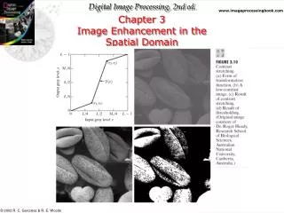
L-1 (r2,s2) s (r1,s1) 0 r L-1 4.2.1 Some Simple Intensity Transformations…(2) • 2. Contrast stretching • (1) Stretching is useful for improving image contrast. • (2) General transformation diagram. L-1 = largest g. l.
4.2.1 Some Simple Intensity Transformations…(3) • (3) cases : • a. no change -- if r1 = s1 , r2 = s2 . • b. thresholding -- if r1 = r2, s1 = 0, and s2 = L-1 ; threshod value = r1 = r2. • c. stretching -- if r1 r2 & s1 s2 ( to keep monotonicity of transformation ) • d. Why dies stretching improve image contrast? • e. How to stretch is problem - dependent
L-1 (r2, s2) =(r0,L-1) T(C) s S=T(r) T(B) (r1, s1) =(r0,0) T(A) r r0 L-1 0 0 A B C 4.2.1 Some Simple Intensity Transformations…(4) Mappings: A=>T(A) (longer => smaller) L-1 = largest g. l. B => T(B) (smaller => larger ) CONTRAST IMPROVED) C => T(C) (larger => smaller)
4.2.1 Some Simple Intensity Transformations…(5) • 3. Compression of dynamic ranges • (1) Gray levels may be out of the display range after certain transformations. • (2) One way to compress is S = T( r ) = c log(1+ | r | ) • where c is a constant to make s to lie between 0 and L-1
4.2.1 Some Simple Intensity Transformations…(6) • 4. Gray level slicing • (1) Highlighting a specific g. l. range • (2) Useful for many applications. • (3) Two approaches: • a. use high values for desired ranges and low values for others; • b. use high values for desired ranges and keep the values for others. • (4) See Fig 4.7
4.2.1 Some Simple Intensity Transformations…(7) • 5. Bit-plane slicing • (1) Highlighting “ contributions made by specific bits to image appearance. • (2) More important information is included in higher- order bit planes; details in others (see Fig. 4.8 ) • (3) Bit - plane 7 ( highest - order ) = result of thresholding with threshold = 128 • (4) See Fig. 4.9
Nk/n …. r 1 2 3 k L-1 4.2.2Histogram Processing…(1) • 1.Definition and properties of histogram • (1) the histogram of a given image f is a function P( rk ) = nk / n where rk = the kth g. l.; nk = the no. of pixels with g.l. rk n = the total no. of pixels in f. • (2) Diagram of histogram
4.2.2Histogram Processing…(2) • (3) Concept : histogram = p.d.f ( probability density function ) • (4) A histogram gives the global appearance of an image . • (5) Histograms of images with high and low contrasts (see Fig. 4.10 )
4.2.2Histogram Processing…(3) • 2. Histogram equalization • (1) Equalization transformation of a given image f : where Pr(w) is the histogram of f • (2) S above is exactly the c. d. f. of r ( c. d. f. = cumulative distribution function )
4.2.2Histogram Processing…(4) • (3) It can be shown by probability theory (see textbook) that the new image with g. l. s has a uniform distribution, i.e., • (4) the transformation illustration Pr(r) Ps(s) Equalization r S Image with low contrast Image with higher contrast
4.2.2Histogram Processing…(5) • (5) Read the example in pp. 176-177. • (6) Histogram equalization is also called histogram flatting or linearization. • (7) Discrete form of histogram equalization
1 2 3 4 5 6 7 4.2.2Histogram Processing…(6) • (8) A computation example 1 3 9 17 23 24
4.2.2Histogram Processing…(7) • (9) A major advantage of histogram equalization for image contrast enhancement is that it can be applied automatically. • (10) See Fig. 4.14 for a real example. • 3. Histogram specification • See textbook • 4. Local enhancement • See textbook
4.2.3Image Subtraction • 1. Computes the difference g of two images f and h : • 2. For application example, see Fig. 4.17
4.2.4Image Averaging • 1.Reduces noise by averaging several copies of and identical image • 2. Method : where gi(x, y) is one of copies of origin image • 3. Why work ? Noise standard deviation can be reduced to 1/n of origin • 4. See Fig. 4.18
4.3Spatial Filtering • 4.3.1 Background • 4.3.2 Smoothing Filtering • 4.3.3 Sharpening Filtering
4.3.1 Background…(1) • 1. Spatial filtering is also called mask processing. • 2. Masks ( also called spatial filters ) are used • 3. High - frequency components in images: • noise, edges, sharp details, etc. • 4. Low - frequency components in images: • uniform regions, slow - changing background g. l., etc. • 5. Type of spatial filtering : • (1) lowpass filtering • useful for image blurring (smoothing)
4.3.1 Background…(2) • (2) Highpass filtering • useful for image sharpening • (3) Bandpass filtering • mostly used in image restoration • 6. See Fig 4.19 for the above 3 types. • 7. Linear mask operation :
4.3.1 Background…(2) • Operation : replace z5 by • R = MN = z1w1 + z2w2 +……. + z9w9 • 8. Nonlinear mask operation : • R is computed nonlinearly using information of the neighborhood of current pixel as well as the mask. Z5 = g. l. of current pixel Mask M Neighborhood N
4.3.2Smoothing Filters…(1) • 1. Used for image blurring & noise reduction. • 2. Useful for removing small details and bridging small gaps in lines or curves. • 3. Lowpass spatial filtering : • (1) Mask for 33 neighborhood
4.3.2Smoothing Filters…(2) • (2) Operation -- replace z5 by • (3) Also called neighborhood averaging • (4) See Fig. 4.22 for effect • 4. Median filtering • (1) Reducing noise without blurring images
4.3.2Smoothing Filters…(3) • (2) Operation -- • replace g. l. at (x, y) with the median of all the g. l. of neighborhood. • (3) Meaning of median • value r such that • (i.e., r = (1/2)tile of the p.d.f. ) P(x) r = median x Area = 1/2
4.3.2Smoothing Filters…(4) • (4) An example: given g. l. z5 = 15 is replaced by median = 20 • (5) For effect of median filtering, see Fig. 4.23
4.3.3Sharpening Filters…(1) • 1. Objective • highlighting or enhancing fine details in images. • 2. Applications • (1) electronic printing; • (2) medical imaging; • (3)industrial inspection; • (4) target detection; • etc.
4.3.3Sharpening Filters…(2) • 3. Basic highpass spatial filtering (HPSF) • (1) Mask for 33 neighborhood • (2) See Fig. 4.25 for effect of filtering • 4. High best filtering • (1) Also called high-frequency emphasis filtering.
4.3.3Sharpening Filters…(3) • (2) Method : high-best = A (original) - lowpass = (A-1)(original) + original - lowpass = (A-1)(original) + highpass where A is a selected weight. • (3) Note that part of the original image is added back. • (4) Equivalent mask • (5) See Fig. 4.27 (A=1.1 is enough) Where w=9A-1 (A =1 basic HPSF)
Averaging (integration) Difference (differentiation) Blurring Sharpening 4.3.3Sharpening Filters…(4) • 5. Derivative filters • (1) Concept - • (2) The most common differentiation operation is the gradient
4.3.3Sharpening Filters…(5) • (3) Gradient • a. definition -- the gradient of a function f at a pixel (x0, y0) is • b. magnitude of gradient --
4.3.3Sharpening Filters…(6) • (4) Approximation of gradient magnitude : • a. Assume the neighborhood (nbhd) g. l. of the pixel at (x, y) are • b. in continuous form With g. l. at (x, y) = z5 or
4.3.3Sharpening Filters…(7) • C. in absolute difference form : • d. Roberts operators for 2 2 nbhd : operation = | N MR1 | + | N MR2 | = | z5-z9 | + | z6 - z8 | or MR1 MR2
4.3.3Sharpening Filters…(8) • d. Prewitt operators for 3 3 nbhd : operation = | N MP1 | + | N MP2 | = | (z7+z8+z9) - (z1+z2+z3) | = | (z3+z6+z9) - (z1+z4+z7) | • e. Sobel operators for 3 3 nbhd : operation = | N MS1 | + | N MS2 | = | (z7+2z8+z9) - (z1+2z2+z3) | = | (z3+2z6+z9) - (z1+2z4+z7) | MP1 MP2 MS1 MS2
4.4 Enhancement in Frequency Domain • 4.4.1 Lowpass Filtering • 4.4.2 Highpass Filtering • 4.4.3 Homomorphic Filtering
4.4.1 Lowpass Filtering…(1) • 1. Use • image blurring ( smoothing ) • 2. Goal • Want to find a transfer function H(u, v) in the frequency domain to attenuate the high frequency in the FT F(u, v) of a given image f using the inverse FT
4.4.1 Lowpass Filtering…(2) • 3. Ideal lowpass filter (ILPF) • (1) Definition -- H(u, v) = 1 if D(u, v) D0 = 0 otherwise where D(u, v) = distance from (0, 0) to (u, v); and D0 is a constant ( called cutoff frequency ) • (2) See Fig 4.30 for the filter shape in 3-D and 2-D • (3) The ILPF cannot be implemented by analog hardware ( but can be implemented by software ) • (4) Before seeing effects of the ILPF, we need to review more properties of the FT first.
4.4.1 Lowpass Filtering…(3) • 4. Additional review of the Fourier transform • See sec.3.2~3.4 for FT, DFT, FFT • See Fig. 4.31 for an example of Fourier spectrum ( or simply called spectrum ) • 5. See Fig. 4.32 for effects of applying the ILPF using different cutoff frequencies. • 6. The ILPF produces ringing effects; see Fig. 4.32(d) for an example; and see Fig. 4.33 for the reason. Note Fig. 4.33(a) is equivalent to the top view of a 2-D sinc function.
4.4.1 Lowpass Filtering…(4) • 7. Butterworth lowpass filter ( BLPF )] • (1) A BLPF of order n with cutoff frequency at D0 is defined as • where A = 1 or 0.414 • (2) See Fig. 4.34 for the shape of the BLPF. • (3) See Fig. 4.35 for the effects of applying the BLPF with n = 1 for 5 D0 values. • 8. The BLPF produces no ringing effect due to the smoothness of its transfer function where A=1 or 0.414
4.4.2 Highpass Filtering…(1) • 1. Use • Image sharpening • 2. Ideal highpass filter (IHPF) • (1) Transfer function H(u, v) = 0 if D(u, v) D0 = 1 otherwise • (2) See Fig. 4.37 for shapes of the IHPF.
4.4.2 Highpass Filtering…(2) • 3.Butterworth highpass filter (BHPF): • (1) Transfer function where A = 1 or 0.414 • (2) See Fig. 4.38 for shapes of the BHPF. • 4.4.3 Homomorphic Filtering • 4.5 Generation of spatial masks from frequency domain specifications • Read the textbook