Download
1 / 27
280 likes | 410 Vues
From Images to Photometric Redshifts. Beatriz Ramos. Introduction. Single Passband (SPB) Catalogs. 1 27.93 26.68 26.22 2 23.85 23.62 23.21 3 27.74 26.59 26.22 4 27.05 25.70 25.20 5 27.58 26.50 26.22 6 26.40 25.75 25.21 7 27.91 26.74 26.22 8 27.04 25.99 25.21

E N D
From Images to Photometric Redshifts Beatriz Ramos
Introduction Single Passband (SPB) Catalogs 1 27.93 26.68 26.22 2 23.85 23.62 23.21 3 27.74 26.59 26.22 4 27.05 25.70 25.20 5 27.58 26.50 26.22 6 26.40 25.75 25.21 7 27.91 26.74 26.22 8 27.04 25.99 25.21 9 23.58 23.29 23.21 10 25.13 24.71 24.21 1 27.93 26.68 26.22 2 23.85 23.62 23.21 3 27.74 26.59 26.22 4 27.05 25.70 25.20 5 27.58 26.50 26.22 6 26.40 25.75 25.21 7 27.91 26.74 26.22 8 27.04 25.99 25.21 9 23.58 23.29 23.21 10 25.13 24.71 24.21 Color Catalogs 1 27.93 26.68 26.22 2 23.85 23.62 23.21 3 27.74 26.59 26.22 4 27.05 25.70 25.20 5 27.58 26.50 26.22 6 26.40 25.75 25.21 7 27.91 26.74 26.22 8 27.04 25.99 25.21 9 23.58 23.29 23.21 10 25.13 24.71 24.21 1 27.9326.68 26.22 2 23.85 23.62 23.21 3 27.7426.59 26.22 4 27.0525.70 25.20 5 27.58 26.5026.22 6 26.4025.75 25.21 7 27.9126.74 26.22 8 27.0425.99 25.21 9 23.5823.2923.21 10 25.13 24.71 24.21 Include Flags: galaxy/star classification, masks over bright objects... Photometric Redshift
Creating SPB Catalogs • SExtractorbuilds a catalog of objects from an astronomical image: • input files: image, configuration parameters and output catalog parameters • methods:single or double image mode image1used for detection of objects and image2for measurements only Depends on the method for the color catalog creation • locate objects • calculate their magnitudes and errors • provide other parameters (ex: related to the reliability of these results) Run SExtractor on images • Information can be added to help with important issues: • classification of objects found as galaxies or stars • delimitation of regions around bright objects (by masks) Catalogs in each observed filter
Improving SExtractor Output Catalogs • Galaxy/Star classification: • simplest: stars = objects with Class_Star > 0.9 and mag < limiting mag • based in Class_Star and Flux_Radius: see Bruno Rossetto’s presentation R R
Improving SExtractor Output Catalogs • Creation of masks around bright/saturated objects : • necessary to avoid objects with contaminated magnitudes • methods: • automatic: see Bruno Rossetto’s presentation • by hand: using DS9 # Region file format: DS9 version 4.0 # Filename: /cosmoinfra/data/DPS/optical/images/Deep2/EIS.2005-12-09T22:58:22.340.fits global color=green font="helvetica 10 normal" select=1 highlite=1 edit=1 move=1 delete=1 include=1 fixed=0 source fk5 polygon(53.634173,-27.633521,53.625467,-27.640746,53.633623,-27.648326,53.642779,-27.640707)
Ok Not Ok
Creating Color Catalogs • Created by the association of objects from SPB catalogs in different filters: SExtractor on single image mode SExtractor on double image mode Association by position (search radius) Direct association using position in a reference image 1 filter Combined Chi2 image (Chi squared sum of images in 3 filters ) • Final catalog with all objects detected in all filters • Difficulties in associating objects: • an object detected in a band, may not be in another one • more than one object close to the same position (multiple associations) • Association is easier, but objects could be missing in the final catalog (an object detected in a filter, may not be in another) Chi2 image minimizes this effect
Data Pruning • Selecting only objects: • located outside masked regions
Data Pruning • Selecting only objects: • located outside masked regions • located away from the images’ borders • that don’t have more than 1 association (in other words, that don’t have more than 1 object associated to a position) only for SExtractor run in single image mode • that are considered reliable by SExtractor • Galaxy/Star classification: • follow object classification in the SPB catalog of a given filter (ex: the one with the best seeing or the deepest one) • use template fitting program (Le Phare) • use color-mag and color-color space (Basílio’s code, Trilegal)
Photometric Redshift • The concept come from Baum (1962), but the interest in it increased more recently, with the higher number of deep multicolor photometric surveys available • Basically needs photometry in 3 filters, with which tries to identify strong spectral features (breaks) • Comparison with spectroscopic redshift: • Advantage: estimates redshift for a greater number of objects per observed area and time • Disadvantage: its precision is worse (more filters and/or better photometric errors can improve it, although this implies in an increase in observation time) • Methods: Fitting of observed Spectral Energy Distribution (SED) by synthetic or empirical template spectra Empirical training set (using spectroscopic redshift sample) Make no assumption concerning galaxy spectra or evolution More simple and does not need spectroscopic sample
Photometric Redshift • Template Fitting: Color catalog + SEDs Templates Hyperz Le Phare • Compare observed magnitudes in different filters with those expected by different SEDs templates look for best 2 fit • Only objects detected in at least 3 filters (higher number of observed filters better fit) UB V R IJ Ks
Hyperz Le Phare • Released version works with galaxy templates, but there is newer version with QSO’s also (http://www.ast.obs-mip.fr/users/roser/hyperz/) • Sequence: • Preparation Phase: • write filter file with selected filters • write template file with selected SEDs: different types of galaxies • Run photo-z program on observed catalog • Input files: color catalog (in a given format) and configuration parameters • Released version works with galaxy, stellar and/or QSO templates • Sequence: • Preparation Phase: • create filter file with selected filters • generate SED library with selected SEDs : galaxy, stellar and/or QSO • build theoretical magnitudes: galaxy, stellar and/or QSO • Run photo-z program on observed catalog • Input files: color catalog (in a given format), configuration parameters and output catalog parameters • Hybrid method: can use a spectroscopic z training set
1+zs Le Phare Ilbert et al 2006 CFHTLS-VVDS photometry (ugriz BVRI JK) CFHTLS-VVDS photometry + VVDS spec-z distribution for calibration
Photometric Redshift • Scatter in photo-z is sensitive to: • number of filters Bolzonella et al 2000
Photometric Redshift • Scatter in photo-z is sensitive to: • number of filters • photometric errors Bolzonella et al 2000
Photometric Redshift • Scatter in photo-z is sensitive to: • number of filters • photometric errors • spectral type Balmer break is weaker for later types Ilbert et al 2006
Photometric Redshift • Scatter in photo-z is sensitive to: • number of filters • photometric errors • spectral type • magnitude Ilbert et al 2006
Artificial Neural Networks (ANNz) • Use spectroscopic z to prepare a training set, used to find z as a function of magnitude This relation is applied to a data set (magnitudes only) determine photo-z Photometric Redshifts for the DES and VISTA and Implications for Large Scale Structure Banerji et al. 2008 • Simulations from different sources (see paper) with DES+VHS filters • Inclusion of NIR filters improvement in : • 0.20 (z>1) and 0.13 (all z) for DES only • 0.15 (z>1) and 0.11 (all z) for DES+VHS Scatter = <(zspec - zphot)2 >1/2 5000 galaxies
Artificial Neural Networks (ANNz) • low z: lack of u filter • high z: improved when NIR is used Banerji et al. 2008
Future Work • Run Hyperz and Le Phare for DES simulated catalogs • Test Annz • Make comparison of the results from the different photo-z programs References • Papers: • Photometric Redshifts for the Dark Energy Survey and VISTA and Implications for Large Scale Structure:Banerji et al.; 2008, arXiv:0711.1059 • Accurate photometric redshifts for the CFHT legacy survey calibrated using the VIMOS VLT deep survey: Ilbert, O. et al.; 2006, A&A 457, 841 • ANNz: Estimating Photometric Redshifts Using Artificial Neural Networks: Collister, A.A.; Lahav, O.; 2004, PASP 116, 345 • Photometric redshifts based on standard SED fitting procedures: Bolzonella, M.; Miralles, J.-M.; Pelló, R.; 2000, A&A 363, 476 • On Twiki: • Photometric Redshift: http://twiki.on.br/bin/view/DesBrazil/PhotometricRedshift • Software Tools: http://twiki.on.br/bin/view/Astrosoft/SoftTools • Des Lectures: http://twiki.on.br/bin/view/DesBrazil/DesLectures • Des Simulations: http://twiki.on.br/bin/view/DesBrazil/DesSimulations
DES simulation v1.03 (5years) – ANNz: cut-off in photo-z=1.5 comes from training set Scatter = <(zspec - zphot)2 >1/2
DES simulations v1.00 (galaxies in 5years of observations): ~4.3million objects
DES sim (5years) – ANNz (from paper): ~930000objects griz DES sim (5years) – ANNz (from WG): ~2.5million objects ~1000objs with err > 1 grizYJHK ~2900objs with err > 1 • Error depends on the noise on the neural network inputs, not on the difference between photo-z and spec-z.