Download
1 / 15
150 likes | 275 Vues
This study examines the seasonal evolution of salinity variations and the South Pacific Eastern Subtropical Mode Water (SPESTMW) through modeling approaches. It explores the role of potential vorticity, Turner angle, and double-diffusion in shaping the salinity distribution. The analysis reveals significant salinity changes influenced by advection and incorporates a simple 1-D model to assess the development of salinity anomalies. Our findings highlight the complexities of salinity flux estimates and the role of double diffusion in the Gulf Stream's salinity dynamics.

E N D
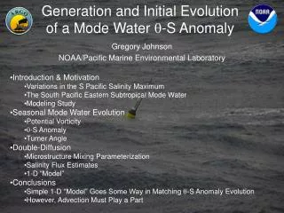
Introduction & Motivation • Variations in the S Pacific Salinity Maximum • The South Pacific Eastern Subtropical Mode Water • Modeling Study • Seasonal Mode Water Evolution • Potential Vorticity • -S Anomaly • Turner Angle • Double-Diffusion • Microstructure Mixing Parameterization • Salinity Flux Estimates • 1-D “Model” • Conclusions • Simple 1-D “Model” Goes Some Way in Matching -S Anomaly Evolution • However, Advection Must Play a Part Generation and Initial Evolution of a Mode Water -S Anomaly Gregory Johnson NOAA/Pacific Marine Environmental Laboratory
SE Pacific Salinity Max Variations Figures after Kessler (1999) S max Subducted in SE Pacific S max Advected Towards Equator • Significant -S Variation along 165E • Salinity Changes of Order 0.4 • Few Locations so Well Measured • Variations Related to Advection • Difficult to Find Cause at Source • Next cut along 103W . . .
South Pacific Eastern Subtropical Mode Water After Wong & Johnson (2003) WOCE P18 Section Data Along 103W in 1994 Region of Small d/dz 25.6 < < 24.8 kg m-3 • Region Sits Below S Maximum • Formed in High E-P Region • Winter Evaporation & Cooling • dS/dz Also Reduced Here • Note dS/dz Destabilizing • Warm Salty Over Cold Fresh
SPESTMW (Continued) After Wong & Johnson (2003) Potential Vorticity Minimum Capped Over in Austral Fall Spreads Equatorward of Formation Region Wide -S Property Range • High Turner Angle • Winter Evaporation & Cooling • Warm Salty Over Cold Fresh • (Tu > 77 = Density Ratio < 1.6) • Potential for Double Diffusion • Just Austral Fall Data • Well After Subduction
Figures of Yeager & Large (2004) • Look on = 25.5 kg m-3 • RMS S (10-2 PSS-78) • Strong Signal In SPESTMW • Propagates Equatorward • Linked to Spiciness Modeled -S Variability • Follow Anomaly Equatorward • Subducted Around 1967-1968 • On Equator 6-7 Years Later • Reduced in Magnitude • Appropriate Diffusivity? • Numerical & Parameterized • Double Diffusion not Enabled . . .
After Johnson (in press) • Just Downstream of High Turner Angle (Spicy) SPESTMW Formation Region • Winter Surface Waters Contoured as 1.0 < R < 2.0 at 0.2 Intervals • WMO IDs 4900451 (cyan) & 4900454 (magenta) • -Deployed January 2004 & Analyzed into July 2005 • -Profiles Every 10 days • -71 Data Points • 100-dbar Spacing at 2000 dbar • Reduces to 8-dbar Spacing by 160-dbar Floats as a Time-Series
Mar 2004 (Black o’s) • Typical of Central Waters • Salinity Destabilizing • Anomaly Near 24.8 kg m-3? • Oct 2004 (Magenta +’s) • Maximum Ventilation • Mixed Layer to 25.0 kg m-3 • Temp Cold But . . . • Upper -S Pulled Salty • < 25.2 kg m-3 • Cooling with Evaporation • Mar 2005 (Cyan ◊’s) • Austral Fall Stratification • Strong Anomaly • Near 25.0 kg m-3 • Anomaly Also Denser • > 25.2 kg m-3 • Double Diffusion? • Downward S Flux • Rotated -S Curve A Condensed Preview of the Time-Series
Potential Vorticity Time-Series Seasonal Mixed Layer Evolution Deeper & Denser Mar-Oct Abrupt Spring Restratification Gradually Lighter Until Fall Maximum Spring Ventilation Pr > 150 dbar ≈ 25.0 kg m-3 • Late Spring PV Reset • Low PV Replenished • 2004 Ventilation vs. 2003 • PV Min Lower • PV Min Thicker • Stronger Ventilation?
Salinity Anomaly Time-Series Pick Reference -S Curves (Blue Vertical Lines) S Anomalies Relative to Curves S Anomaly Around 0.3 PSS-78 Salty & Warm Water Subducted • Subsequent Evolution • Max Anomaly Reduces • Anomaly Also Moves Denser • Result of Salt-Fingering? • Patchiness • Mesoscale? • Advection? • Winter 2004 Stronger Than 2003?
Turner Angle Time-Series Contours: R ≤ 2.0 at 0.1 intervals Wintertime Latent Cooling with . . . Strong Evaporation Salinity Anomaly Favors Large Turner Angle Double Diffusion • Seasonal Anomaly Evolution • Again Tu Maximum Eroded • Migrates Downward • Similar to the S Anomaly • Interannual Variations • 2004 Exceeds 2003
Parameterize Salt Fingering Mixing Use an Ad-Hoc Parameterization Decreased Stability ->Increased Mixing After Yeager & Large (2004, Eq. B1) St. Laurent & Schmitt (1999) Data Assume That For 1 < R < 2.05 (90 < Tu < 71): Ks (R) = 2.410-4 F + 0. 110-4 m2 s-1 With F = [1 - (R - 1)/(2.05 - 1)]3 And Elsewhere: Ks = 0.110-4 m2 s-1
Use Previous Parameterization • Admittedly Ad-Hoc & Uncertain • Salinity Flux Below S Anomaly • Large Diapyncal Flux Downward • Significant Fraction of Anomaly Size Over a Year Diapycnal Salinity Flux Time-Series • Seasonal Anomaly Evolution • Flux Decays with Time • Zero-Crossing Denser with Time • Similar to Other Fields • Interannual Variations . . . • 2004 Stronger than 2003 • Next: Follow = 25.35 kg m-3
Model S Anomaly on = 25.35 kg m-3 Find Diapycnal Salt Flux on Isopycnal Integrate with Time (1-D) Compare Mapped Salinities Pick Best Agreement Integration Constant • Seasonal Anomaly Evolution • Anomaly Ramps up in Spring • Decays slowly thereafter • Delayed for 4900454 • Weaker Northern Winter Ventilation
1-D Model is Surprisingly Good • However, Advection is Present • Short-term Variations (Eddies) • Mean Circulation • Mixed Layer Slumping? • In January 2004 Data Were Few • Difficult Even to Map Anomaly • More Difficult to Trace Anomaly • In January 2006 Data Are Many • Anomaly Mapping & Tracing Almost Possible? What about Advection?
Observational and Modeling Studies Reveal SE Pacific -S Variations • Warm Salty Water Subducted in SE Subtropical Pacific • Spiciness Enables Large -S Variation in Eastern STMW • Anomalies May Even Reach the Equator, Upwell, and Influence SST • Argo Floats Allow Local Studies of Seasonal Mode Water Evolution • Potential Vorticity • -S Anomaly • Turner Angle • Double-Diffusion May Be Important • Microstructure Mixing Parameterization • Salinity Flux Estimates from 1-D “Model” Match Observations Pretty Well • Advection Must Play a Role Over Longer Time-Scales • Next Steps: Mapping Anomalies & Tracing Their Evolution • Growth of Array Begins to Make this Realistic • Requires Data From a Continuous Argo Float Array • Must Maintain Array over Several Years • For Mapping Anomalies & Tracing Them Equatorward • For Analyzing Interannual Variations Conclusions