Binomial Distribution: Application and Analysis
140 likes | 177 Vues
Explore the fundamentals of the binomial distribution, its parameters, and practical examples such as blood types, card dealing, and more. Learn how to calculate probabilities, simulate experiments, and determine unusual outcomes.

Binomial Distribution: Application and Analysis
E N D
Presentation Transcript
8.1 The Binomial Distribution • Definition: “The Binomial Setting” : A situation is said to be a “BINOMIAL SETTING”, if the following four conditions are met: • Each observation is one of TWO possibilities - either a success or failure. • There is a FIXED number (n) of observations. • All observations are INDEPENDENT. • The probability of success (p), is the SAME for each observation.
8.1 The Binomial Distribution • Definition: “Binomial Distribution” • The distribution of the count X of successes in the binomial setting is the BINOMIAL DISTRIBUTION with parameters n and p. • n = the number of observations • p = the probability of success on any one observation • A way to symbolically say this: B(n, p)
8.1 The Binomial Distribution • Example 8.1: BLOOD TYPES • Example 8.2: DEALING CARDS • Example 8.3: INSPECTING SWITCHES • Example 8.4: AIRCRAFT ENGINE RELIABILITY
8.1 The Binomial Distribution • Finding Binomial Probabilities • We will use the TI-83/4 • We will use a “by-hand” formula • Example 8.5: INSPECTING SWITCHES • SRS of 10 switches from a LARGE shipment • 10% of the switches are “bad” • P(No more than 1 of the 10 switches are “bad”) • Draw a Probability histogram (on TI-8X) • Binompdf(n, p, X) and Binomcdf(n, p, X)
8.1 The Binomial Distribution • Example 8.6: CORRINE’S FREE THROWS • 75% lifetime free-thrower • 12 shots in a key game were takes, and ONLY 7 made … Is this “unusual”? • FIST? • P(X<=7) = ?
8.1 The Binomial Distribution • Example 8.7: THREE GIRLS • Find P(X = 3) • L1 = {0, 1, 2, 3} L2 = binompdf (3, .5, L1) • Plot1…On…Histogram • Xlist:L1 Freq:L2 • WINDOW: Xmin: -.5 Xmax: 3.5 Ymin: -.1 Ymax: .4 • Xlist:L1 Freq:L3 L3 = binomcdf (3, .5, L1) • WINDOW: Ymax: 1.1 • Graph
8.1 The Binomial Distribution • Example 8.8: IS CORINNE IN A SLUMP? • Same 75% free-thrower • Let’s create both the probability distribution and the cumulative distribution functions. • L1 = {0, 1, 2, … 10, 11, 12} • L2 = binompdf (12, .75, L1) L3 = binomcdf (12, .75, L1) • Xlist:L1 Freq:L2 • WINDOW: Xmin: -.5 Xmax: 12.5 Ymin: -.1 Ymax: .3 • Xlist:L1 Freq:L3 L3 = binomcdf (3, .5, L1) • WINDOW: Ymax: 1.1 • Graph
8.1 The Binomial Distribution • Example 8.9: INHERITING BLOOD TYPE • Each child in a family has probability of .25 of having blood type O. • P(X = 2) • FIST? • List by hand all S-F configuration for 2 S’s in a family of 5. • Find each probability … multiply by how many ways it an occur
8.1 The Binomial Distribution • The binomial coefficient: An alternative to listing all 10 options from the previous example. • The number of ways of arranging k successes among n observations is given by: Example:
8.1 The Binomial Distribution • The Binomial Probability Formula • If X has the binomial distribution with n observations and probability p of success on each observation, the possible values of X are 0, 1, 2, …, n. If k is any one of these values, Example 8.10: DEFECTIVE SWITCHES Part 2
8.1 The Binomial Distribution • The Binomial Mean and Standard Deviation Example 8.11: DEFECTIVE SWITCHES Part 3
8.1 The Binomial Distribution • The Normal Approximation to the Binomial Distribution – when n is “large” … Rule of Thumb: Example 8.12: ATTITUDES TOWARDS SHOPPING Sample size n = 2500; p = .6 “Agree – I like buying new clothes, but shopping is often frustrating and time-consuming” P(X >= 1520) 1 – binomcdf(2500, .6, 1519) … or … Get mean, standard deviation, and then z, and normalcdf
8.1 The Binomial Distribution • Simulating Binomial Experiments • Example 8.14: CORINNE’S FREE THROWS • p = .75 … n = 12 … P(X <= 7) = 0.1576 • randBin(1, .75, 12) • randBin(1, .75, 12)L1:sum(L1) • Simulate 20 games … Compare to .1576 • Get class average. Does Law of Large numbers take over?