
Association Rules Mining: Concepts and Applications
E N D
Presentation Transcript
Association Rules Berlin Chen 2005 References: 1. Data Mining: Concepts, Models, Methods and Algorithms, Chapter 8 2. Data Mining: Concepts and Techniques , Chapter 6
Association Rules: Basic Concepts • A kind of local pattern discovery which operates in an unsupervised mode • Mine gold (a rule or interesting pattern) through a vast database that is not already known and not explicitly articulated • Intratransaction association rules • Given: • Database of transactions • Each transaction is a list of items (purchased by a customer in a visit) • Find: • All rules that correlate the presence of one set of items with that of another set of items • E.g., 98% of people who purchase tires and auto accessories also get automotive services done
What Is Association Mining? • Association rule mining: • Find frequent patterns, associations, correlations, or causal structures among sets of items or objects in transaction databases, relational databases, and other information repositories • Applications: • Basket data analysis, cross-marketing, catalog design, loss-leader analysis, clustering, classification, etc. • Examples. • Rule form: “Body → Head [support, confidence]”. • buys(x, “diapers”) → buys(x, “beers”) [0.5%, 60%] • major(x, “CS”) ^ takes(x, “DB”) → grade(x, “A”) [1%, 75%]
Application: Market Basket Analysis (cont.) • Market Basket • A collection of items purchased by a customer in a single transaction • A well-defined business activity • Market Basket Analysis • Accumulate huge collections of transactions to find sets of items (itemsets) that appear together in many transactions • A itemset consists of i items is called i-itemset • The percentage of transactions that contain an itemset is called the itemset’s support (high support →high frequency → interesting !) • Use knowledge of obtained patterns to improve • The placement of items in the store • The layout of mail-order catalog pages and Web pages
Measures: Support and Confidence • Find all the rules X ∩ Y Z with minimum confidence and support • Support, s, probability that a transaction contains {X ∩ Y ∩ Z} • Indicate the frequency of the pattern • Confidence, c, conditional probability that a transaction contains {X ∩ Y} also contains Z • Denote the strength of implication • Example: Let minimum support 50%, and minimum confidence 50%, we have • A C (50%, 66.6%) • C A (50%, 100%) Quantities of items bought are not considered here
Mining Association Rules: Task Definition • Discover strong association rules in large databases • Strong association rules: such rules with high confidence and strong support • Problem of association rule mining can be decomposed into two phases • Discover the large (frequent) itemsets that have transaction support above a predefined minimum threshold • How to efficiently compute the large frequent itemsets is critical • Use the obtained large itemsets to generate the association rules that have confidence above a predefined minimum threshold support as the criterion confidence as the criterion
Mining Association Rules: Example Min. support 50% Min. confidence 50% • For rule AC: support = support({A∩C}) = 50% confidence = support({A∩C})/support({A}) = 66.6%
Apriori Algorithm • Discover large (frequent) itemsets in the database • Iteratively compute the frequent itemsets with cardinality from 1 to M (M-itemset) • Then use the frequent itemsets to generate association rules • Each iteration i compute all frequent i-itermsets • Step 1: Candidate generation (joint step) • Ck(candidate itemsets of size k)is generated by joining Lk-1(frequent itemset of size k-1 ) with itself • Or more specifically,
Apriori Algorithm (cont.) • Step 2: Candidate counting and selection (prune step) • Any (k-1)-itemset that is not frequent cannot be a subset of a frequent k-itemset • In other words, an itemset is frequent if all its subsets are frequent as well • Search through the whole database (count support) E.g., {A, B, C} is a frequent itemset if {A, B}, {A,C}, {B, C} are frequent
Apriori Algorithm: Example • Transactional data for an AllElectronic branch minimum support count = 2
Apriori Algorithm: Example • Because there is no candidate 4-itemset to be constructed from L3, Apriori ends the iterative process
Discovering Association Rules from Frequent Itemsets • Systematically analyze all possible association rules that could generated from the frequent itemsets and then select rules with high confidence values • A rule implies x1∩x2∩x3x4 • Both itemsets {x1,x2,x3,x4} and {x1,x2,x3} must be frequent • Confidence c of the rule is computed as: • c = support(x1∩x2∩x3∩x4)/support(x1∩x2∩x3) • c should be above a given threshold • Example • B∩C E • c=support(B∩C∩E)/support(B∩C)=2/2=1 • B∩E C • c=support(B∩C∩E)/support(B∩E)=2/3=0.66
Discovering Association Rules from Frequent Itemsets (cont.) • In general, association rules can be generated as follows • For each frequent itemset l, generate all nonempty subsets of l • For every nonempty subset s of l, output the rule s (l-s) if • Example: for the frequent itemset {I1, I2, I5} • Nonempty subsets: {I1, I2}, {I1, I5}, {I2, I5}, {I1}, {I2}, {I5} • Resulting association rules (if confidence threshold is 70%) • I1∩I2I5 with c=2/4 • I1∩I5I2 with c=2/2 • I2∩I5I1 with c=2/2 • I1I2∩I5 with c=2/6 • I2I1∩I5 with c=2/7 • I5I1∩I2 with c=2/2
Are Strong Rules Interesting ? • Not all strong association rules are interesting enough to be presented and used • E.g.: A survey-result in a school of 5,000 students • 3000 students (60%) play basketball • 3,750 students (75%) eat cereal • 2,000 students (40%) play basketball and also eat cereal • Minimal support (s=0.4) and minimal conference (c=0.6) are set • However, the overall percentage of students eating cereal is 75% is larger than 66% (play basketball) → (eat cereal) (s=0.4, c=0.66) P(eat cereal)> P(eat cereal | play basketball)0.75 0.66 => negative associated !
Are Strong Rules Interesting ? (cont.) • Heuristics to measure association A → B is interesting if • [support(A∩B) / support(A)] - support(B) > d • Or, support(A∩B) - support(A)‧support(B) > k • A kind of statistical (linear) independence test • E.g.: the association rule in the previous example support(play basketball∩eat cereal) - support(play basketball) ‧support(eat cereal) = 0.4 - 0.6‧0.75 = -0.05 < 0 (negative associated !)
Improving Efficiency of Apriori 1. Hashing itemset counts • E.g., generate all of the 2-itemsets for each transaction, andhash (map) them into different buckets and increase the corresponding bucket counts • A itemset whose corresponding bucket count is below the support threshold can not be frequent and thus should be removed x = +
Improving Efficiency of Apriori (cont.) 2. Transaction reduction • A transaction that does not contain any frequent k-itemset is useless in subsequent scans (should be marked or emoved from further consideration) • Cannot contain any frequent k+1-itemset 3. Partition the whole database • Any itemset that is potentially frequent in D must be frequent in at least one of the partitions of D • Local frequent itemsets are candidate itemsets with respect to D
Improving Efficiency of Apriori (cont.) 4. Sampling • Pick a random sample S of D, and then search for frequent itemsets (LS) in S instead of D • Then use the rest of DB to compute the actual frequenciesof each LS • Lower support threshold + a method to determine the completeness 5. Building concept hierarchy • Multilayer association rules
Known Performance Bottlenecks of Apriori • The core of the Apriori algorithm: • Use frequent (k – 1)-itemsets to generate candidate frequent k-itemsets • Use database scan and pattern matching to collect counts for the candidate itemsets • The bottleneck of Apriori: candidate generation • Huge candidate sets: • 104 frequent 1-itemset will generate 107 candidate 2-itemsets • To discover a frequent pattern of size 100, e.g., {a1, a2, …, a100}, one needs to generate 2100 1030 candidates • Multiple scans of database: • Needs (n +1 ) scans, n is the length of the longest pattern scalability problem
Frequent-Pattern (FP) Growth • Mine the complete set of frequent itemsets without the time-consuming candidate generation process • Idea of FP growth • Compress a large database into a compact, Frequent-Pattern tree (FP-tree) structure • Highly condensed, but complete for frequent pattern mining • Avoid costly database scans • Develop an efficient, FP-tree-based frequent pattern mining method • A divide-and-conquer methodology: decompose mining tasks into smaller ones • Avoid candidate generation: sub-database test only!
Frequent-Pattern (FP) Growth (cont.) • Steps to construct FP-tree • Scan DB once, find frequent 1-itemset (single item pattern) • Minimum support count set to 2 here • Order frequent items in frequency/support descending order • Scan DB again, construct FP-tree • FP-tree is a prefix tree • A branch is created for each transaction with frequent items item header table
Frequent-Pattern (FP) Growth (cont.) • Benefits of the FP-tree Structure • Completeness: • Never breaks a long pattern of any transaction • Preserve complete information for frequent pattern mining • Compactness • Reduce irrelevant information—infrequent items are gone • frequency descending ordering: more frequent items are more likely to be shared • Never be larger than the original database (if not count node-links and counts)
Frequent-Pattern (FP) Growth (cont.) • Mine the FP-tree • General idea (divide-and-conquer) • Recursively grow frequent pattern path using the FP-tree • Method • For each item (length-1suffix pattern), construct its conditional pattern-base (subdatabase) and then its conditional FP-tree • Conditional pattern-base: prefix paths in FP-tree co-occurring with the suffix pattern • Prune node or path with low support count in the tree • Repeat the process on each newly created conditional FP-tree • Until the resulting FP-tree is empty, or it contains only one path (single path will generate all the combinations of its sub-paths, each of which is a frequent pattern)
Frequent-Pattern (FP) Growth (cont.) • Mine the FP-tree: Example I3’sconditional- pattern base
Why Is Frequent Pattern Growth Fast? • Previous performance study showed • FP-growth is an order of magnitude faster than Apriori • Reasons • No candidate generation, no candidate test • Use compact data structure • Eliminate repeated database scan • Basic operation is counting and FP-tree building
Mining Multilevel Association Rules • Phenomena • Difficult to find strong associations among data items at low or primitive levels of abstraction due to the sparsity of data in multidimensional space • Strong associations discovered at high concept levels may represent common sense knowledge Concept Hierarchy Here we focus on finding frequent itemsets with items belonging to the same concept level
Mining Multilevel Association Rules (cont.) • Uniform Support: the same minimum support for all levels • Pro: One minimum support threshold. No need to examine itemsets containing any item whose ancestors do not have minimum support • Con: Lower level items do not occur as frequently. If support threshold • too high miss low level associations • too low generate too many high level associations
Mining Multilevel Association Rules (cont.) • Reduced Support: reduced minimum support at lower levels • Each level of abstraction has its own minimum support threshold • The lower the abstraction level, the smaller the corresponding threshold
Mining Multilevel Association Rules (cont.) • Reduced Support: 4 alternative search strategies 1. Level-by-level independent • Each node is examined regardless of whether or not its parent node is found to be frequent • Numerous infrequent items at low levels have to be examined 2. Level-cross filtering by k-itemset • A k-itemset at Level i is examined if and only if its corresponding parent k-itemset at Level i-1 is frequent • Restriction is very strong, so many valuable patterns may be filtered out (computer, furniture) →(laptop, computer chair) (computer, accessories) →(laptop, mouse)
Mining Multilevel Association Rules (cont.) 3. Level-cross filtering by single item • A compromise between “1.” and “2.” • An itemset at Level i is examined iff its parent node at Level i-1 is frequent • May miss associations between low items that are frequent based on a reduced minimum support, but whose ancestors do not satisfy minimum support
Mining Multilevel Association Rules (cont.) 4. Controlled level-cross filtering by single item • A modified version of “3.” • A level passage threshold is set for a given level with between the minimum support value of the next lower level and that of the given level • Allow the children of items that do not satisfy the minimum support threshold to be examined if these items satisfy the level passage threshold
Mining Multilevel Association Rules (cont.) • Redundancy Association Rule Filtering • Some rules may be redundant due to “ancestor” relationships between items. • Example (suppose ¼ sales of desktop computers are IBM) • desktop computer b/w printer [support = 8%, confidence = 70%] • IBM desktop computer b/w printer[support = 2%, confidence = 72%] • We say the first rule is an ancestor of the second rule • A rule is redundant if its support is close to the “expected” value, based on the rule’s ancestor • Do not offer any additional information and is less general than the rule’s ancestor
Multi-Dimensional Association Rules • Rather than simply mining a transactional DB, sales and related information are stored in a relational DB can be mined as well • Multidimensional: each database attribute as a dimension or predicate • Items, quantities and prices of items, customer ages, etc. • Single-dimensional (intra-dimensional) rules: buys(X, “milk”) buys(X, “bread”) • Multi-dimensional rules: ≥ 2 dimensions or predicates • Inter-dimension association rules (no repeated predicates) age(X,”19-25”) occupation(X,“student”) buys(X,“coke”) • hybrid-dimension association rules (repeated predicates) age(X,”19-25”) buys(X, “popcorn”) buys(X, “coke”) predicate/dimension
Multi-Dimensional Association Rules (cont.) • Types of DB attributes considered • Categorical (nominal) Attributes • Finite number of possible values • No ordering among values • Quantitative Attributes • Numeric • Implicit ordering among values • Confine to mining interdimension association rules • Instead of searching for frequent itemsets, here frequent predicate sets (Lk, k-predicate sets) are looked for • E.g., the set of predicates {age, occupation, buys} • Apriori property: every subset of a frequent predicate set must also be frequent age(X,”19-25”) occupation(X,“student”) buys(X,“coke”)