
Governing Equations and Turbulence Closure in Mean Turbulent Flow Analysis
E N D
Presentation Transcript
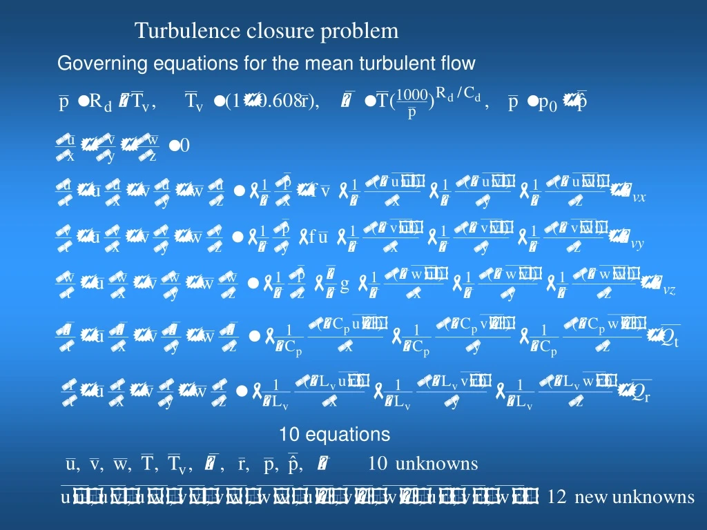
Turbulence closure problem Governing equations for the mean turbulent flow 10 equations
Simplification of governing equations Assumptions: a. Mean vertical velocity is zero. Hydrostatic balance is applied. b. Horizontal turbulent mixing << Vertical turbulent mixing. c. Viscosity is negligible d. Adiabatic process. e. no phase change. f. Horizontal homogeneous
Local turbulence closure z a. First-order closure Turbulent transport x z Turbulent transport x Z
b. How to compute , Prandtl mixing length theory Assuming an air parcel does not change its properties during a displacement associated with an eddy, then, the velocity difference between the air parcel and the environment is, Vertical displacement must be caused by an upward vertical velocity , Assuming, , then, Flux Mixing length
Eddy viscosity Eddy viscosity is determined by the shear, a measure of turbulent intensity, and the mixing length, a measure of mixing ability of turbulence. c. Surface layer (constant flux layer) The layer above the surface in which the change in turbulent fluxes with height is negligible, so, it is also called constant flux layer. The averaged depth is about 20-30 m depending on the turbulent intensity. In the surface layer, the size of turbulent eddies is constraint by the surface, thus, we assume, Frictional velocity Rotating x-axis along the mean wind direction, then,
Above the surface layer, the size of turbulent eddies is not constraint by the surface, thus, mixing length is no longer proportional to height, rather, it is determined by the strength of turbulence via stability and the background winds. d. Monin-Obukhov length L Rotating x-axis along the mean wind direction, In the surface layer, Monin-Obukhov length
Monin-Obukhov length is the height where turbulent shear production balances turbulent buoyancy destruction under stable condition and the height where turbulent shear production balances turbulent buoyancy production under unstable condition. In real applications, we define a non-dimensional height >0, stable =0, neutral <0, unstable Relationship between
Mellor L. G., 1982: Development of a turbulence closure model for geophysical Fluid problems. Reviews of Geophysics and Space Physics. 20 , 851-875. Deardorff, 1980.Strato-cumulus capped mixed layers derived from a three-dimensional model. Boundary-Layer Meteorol. 18 (1980), pp. 495\u2013527. Klemp, J. B., and R. B. Wilhelmson, 1978: The simulation of three-dimensional convective storm dynamics. J. Atmos. Sci., 35, 1070-1096. Moeng, C.-H., 1984: A large-eddy-simulation model for the study of planetary boundary-layer turbulence. J. Atmos. Sci., 41, 2052-2062.
f. Second order and higher order turbulent closure Still consider the simplest case, horizontal homogeneous
To close the system, further assume Third order turbulent closure is to use third-order moments to parameterize fourth-order moments. Fourth order turbulent closure is to use fourth-order moments to parameterize fifth-order moments. ……… Why higher order closure is better than lower order closure? The advantage of higher-order turbulence closure is that parameterizations of unclosed higher-order moments, e.g., fourth-order moments, might be very crude, but the prognosed third-order moments can be precise since there are enough remaining physics in their budget equations. The second-order moment equations bring in more physics, making them even more precise, and so on down to the first-order moments.
Non-local turbulence closure Under convective condition, buoyancy driven convective large turbulent eddies can produce direct mixing over a finite distance, which cannot be described by local down-gradient mixing. Illustration of non-local turbulent mixing concept Entraining in Entraining in 1 1 2 2 Detraining out Detraining out 3 3 4 4 Entraining in Entraining in 1 1 2 2 Detraining out Detraining out 3 3 4 4