Download
1 / 31
320 likes | 446 Vues
Application of Multifractals in WWW Traffic Characterization. Marwan Krunz Department of Elect. & Comp. Eng. Broadband Networking Lab. University of Arizona http://www.ece.arizona.edu/~bnlab krunz@ece.arizona.edu. Presentation Outline. WWW Traffic Monofractals Versus Multifractals

E N D
Application of Multifractals in WWW Traffic Characterization Marwan Krunz Department of Elect. & Comp. Eng. Broadband Networking Lab. University of Arizona http://www.ece.arizona.edu/~bnlab krunz@ece.arizona.edu
Presentation Outline • WWW Traffic • Monofractals Versus Multifractals • Proposed Model • Simulation Results • Ongoing Research • Other BNL Projects
C C C WWW Traffic • What do we mean by WWW traffic? • Sequence of requests for file objects at a server • Why do we want to model it? • Capacity planning & resource dimensioning • Design of caching & prefetching schemes • What traffic properties to capture? • Popularity • Temporal locality • Spatial locality Internet C C C Web server
time A B A C B D A B A C B D A B A C B D A B A 1 3 3 4 4 3 2 stack distance string B A B A C B D A B C C C B A C B D D D D D D D A C C C Stack Temporal Locality • Closeness in time between references to the same object • Often measured using the stack distance string 2 2
Temporal Locality (cont.) • Temporal locality is often represented by the marginal distribution of the stack distance string • Approximately lognormal • Sources of temporal locality: • “Long-term” popularity of objects • Temporal correlations between requests to same object
Temporal Locality (cont.) • Need to differentiate between the two sources, since • Long-term popularity suggests the use of long-term frequency information in caching (LFU) • Temporal correlations suggest the use of short-term residency information in caching (LRU) • Solutions: • Have several, popularity-based stack-distance models • Use a scaled version of the stack distance string [Cherkasova & Ciardo, 2000] • Stack distances normalized by their mean stack distance
Example – CLARKNET Trace Mean stack distance Popularity (# of requests)
Spatial Locality • Correlations between requests to different files • Can be captured through the autocorrelation function (ACF) of the (scaled) stack distance string • Empirical ACF exhibits a slowly decaying behavior; an indication of long-range dependence (LRD)
Example time A B F G E D A H B F E D 6 7 7 Stack distance: 6,7,7,… high autocorrelation value at lag 1 of the stack distance string
How to Simultaneously Capture Temporal and Spatial Localities • Previous approach: Self-similar model (Crovella et al.) • Start with a F-ARIMA with a desired H-parameter • Transform the Gaussian distribution of the F-ARIMA process into a lognormal distribution • Problems: • H-parameter characterizes only the long-term correlation behavior • Transformation is nonlinear (hence, it does NOT preserve the overall structure of the ACF)
Impact of Transformation Autocorrelations F-ARIMA (after transformation) F-ARIMA (before transformation) Real Lag (in stack distances)
Monofractals (Self-Similarity) • Example from geometry: The Sierpinski gasket
Self-similar traffic Poisson traffic Self-Similarity in Network Traffic
Self-Similarity … More Formally • Consider a random process X = {X(t)} with mean , variance v, and ACF R(k), k = 0 , 1, … • Let X(m)be the aggregated process of X over non-overlapping blocks of length m • X is exactly self-similar with scaling factor 0 < H < 1 if
ACF Lag Other Related Definitions • A process Y = {Y(t)} exhibits LRD if it is the derivative process of a self-similar process with H > 0.5 • Manifestations of LRD behavior: • ACF of Y decays hyperbolically • Spectral density obeys a power law near the origin: F()~c -, as 0 • vVariance of the sample mean decreases more slowly than the reciprocal of the sample size
Multifractal Processes • Generalizations of self-similarity, where now the H parameter varies with scale • Wavelet construction of multifractals (Riedi et al.): • Discrete wavelet transform of sequence to be modeled Scale coefficient at scale J and time 2Jk Shifted and translated wavelet function Coarsest scale Shifted and translated scale function Wavelet coefficient at scale j and time 2jk
M A1*M A2*M A3*A1*M A4*A1*M Multifractal Processes (cont.) • Multifractals can be generated using a semi-random cascades: Ai is a symmetric random variable If dependent semi-random cascade
Multifractal Wavelet Model • Trace = scale coefficients at the finest time scale • For the Haar transform, the scale and wavelet coefficients are: 2 1 4 7 Wavelet coefficient Scale coefficient 3/21/2 1/21/2 11/21/2 -3/21/2 14/2=7 -8/2=-4
To generate synthetic data: • Scale coefficients at coarsest scale: U0,0 ~ N(E[U0,0],Var[U0,0]) • Synthetic trace is obtained from the scale coefficients at finest scale where Aj,k, k = 1,2,…, are iid symmetric rvs with mean zero. Let Aj be a generic r.v. having the same CDF as Aj,k Multifractal Wavelet Model (cont.)
Multifractal Wavelet Model (cont.) • Autocorrelations are controlled through the energy at scale j, i.e., E[Wj2] • To produce a synthetic trace with a desired ACF, the parameter(s) of Aj is selected based on: • Problem: Need to compute E[Wj2] for all scales j Large number of model parameters
Modified Multifractal Model • Goal: Reduce the complexity of the original model • Outline of modified model: • Take Aj to be a triangular rv in the range[-cj, cj]for all j • Define the aggregated sequence {Xn(m) : n = 1, 2, …} • Relate E[(Xn(m))2] to E[Uj2] and, thus, to E[Aj2] • Aggregation level 2m represents the scale j-1 • Express cj-1 c(2m) in terms of E[(Xn(m))2] and E[(Xn(2m))2]
Modified Multifractal Model (cont.) • Relate E[(Xn(m))2] to the mean (), variance (v), and ACF (k: k = 1,2,…) of the original trace: • Thus, cj,j = 1, 2, …,is expressed in terms of , v, and k: k = 1,2,… • For the ACF, we use the general form: • g(k) is taken to be k or log(k+1) model is specified using 4 parameters
Outline of Traffic Generation • Extract empirical (scaled) stack distances • Start with an empty stack (to avoid initial ordering problem) • Process trace in the reverse direction • Record stack depth only for objects already in the stack • Reverse the extracted stack distance string • Normalize stack distances by their empirical averages • Generate synthetic stack distance string • Compute parameters for multifractal model • Generate a synthetic (scaled) stack distance string • Scale back stack distances • Generate URL traces while enforcing popularity profile
Scaled back synthetic stack distance string 2 3 4 4 3 4 2 3 C B D B D A A B A C B D A B A D A C B A C B D A B A C A C B C C B D A B C C B A A C B D A B A C B D D D D A C C D D D synthetic traffic Traffic Generation Example Trace length=12 popularity profile: frA=4/12 frB=4/12 frC=2/12 frD=2/12 B
Simulation Results Real Multifractal model
Simulation Results (cont.) Real Multifractal model
Ongoing & Future Work • Online traffic forecasting using multifractal model • Incorporation of traffic forecasting in design of prefetching strategies
Modeling of Prefetching Systems • Goal: Provide a theoretical model to analyze the performance of generic prefetching systems • Limitations of existing works: • Many are mainly focused on the prediction aspect only • Performance is often studied via simulations under very specific setups (e.g., given network topology) • Few analytical models, but which are overly simplistic (e.g., ignore client behavior, TCP dynamics, etc.)
Framework Client: ON/OFF source Should I only use thinking time for prefetching? Predictor: I suggest you prefetch documents: D1,D2,….,Dk since I think they will be requested soon with probabilities: P1, P2, …., Pk. One TCP connection for both, demand fetching and prefetching An access to a prefetched document moves the document to the local cache. This helps in Studying the performance of prefetching in isolation from caching. OR Two separate TCP connections Server Prefetching cache: Small portion of the local cache Local cache