Download
1 / 67
670 likes | 786 Vues
In this lecture from Spring 2000, Prof. Jan Rabaey explores the revolutionary advancements in reconfigurable computing, highlighting major contributions from Andre Dehon. Featuring the latest DSP technologies like TI's C64x and C55x, the discussion emphasizes energy efficiency, performance improvements, and the adaptability of hardware to specific applications. Concepts such as spatial vs. temporal computing, parameterizable hardware, and the benefits and challenges of configurable designs are examined. This lecture serves as a key resource for understanding the evolution of embedded systems and the future of programmable logic.

E N D
Lecture 13: (Re)configurable Computing Prof. Jan Rabaey Computer Science 252, Spring 2000 The major contributions of Andre Dehon to this slide setare gratefully acknowledged
Computers in the News … TI announces 2 new DSPs • C64x • Up to 1.1 GHz • 9 Billion Operations/sec • 10x performance of C62x • 32 full-rate DSL modems on a single chip! • C55x • 0.05 mW/MIPS (20 MIPS/mW!) • Cut power consumption of C54x by 85% • 5x performance of C54x
Components of Cost Area of die / yield Code density (memory is the major part of die size) Packaging Design effort Programming cost Time-to-market Reusability Evaluation metrics for Embedded Systems Power Cost Flexibility Performance as a Functionality Constraint (“Just-in-Time Computing”)
What is Configurable Computing? Spatially-programmed connection of processing elements • “Hardware” customized to specifics of problem. • Direct map of problem specific dataflow, control. • Circuits “adapted” as problem requirements change.
Spatial vs. Temporal Computing Temporal Spatial
Computes one function (e.g. FP-multiply, divider, DCT) Function defined at fabrication time Computes “any” computable function (e.g. Processor, DSPs, FPGAs) Function defined after fabrication Parameterizable Hardware: Performs limited “set” of functions Defining Terms Fixed Function: Programmable:
“Any” Computation?(Universality) • Any computation which can “fit” on the programmable substrate • Limitations: hold entire computation and intermediate data • Recall size/fit constraint
Benefits of Programmable • Non-permanent customization and application development after fabrication • “Late Binding” • economies of scale (amortize large, fixed design costs) • time-to-market (evolving requirements and standards, new ideas) Disadvantages • Efficiency penalty (area, performance, power) • Correctness Verification
Spatial/Configurable Benefits • 10x raw density advantage over processors • Potential for fine-grained (bit-level) control --- can offer another order of magnitude benefit • Locality! Spatial/Configurable Drawbacks • Each compute/interconnect resource dedicated to single function • Must dedicate resources for every computational subtask • Infrequently needed portions of a computation sit idle --> inefficient use of resources
Early RC Successes • Fastest RSA implementation is on a reconfigurable machine (DEC PAM) • Splash2 (SRC) performs DNA Sequence matching 300x Cray2 speed, and 200x a 16K CM2 • Many modern processors and ASICs are verified using FPGA emulation systems • For many signal processing/filtering operations, single chip FPGAs outperform DSPs by 10-100x.
Issues in Configurable Design • Choice and Granularity of Computational Elements • Choice and Granularity of Interconnect Network • (Re)configuration Time and Rate • Fabrication time --> Fixed function devices • Beginning of product use --> Actel/Quicklogic FPGAs • Beginning of usage epoch --> (Re)configurable FPGAs • Every cycle --> traditional Instruction Set Processors
The Choice of the Computational Elements Reconfigurable Logic Reconfigurable Datapaths Reconfigurable Arithmetic Reconfigurable Control Bit-Level Operations e.g. encoding Dedicated data paths e.g. Filters, AGU Arithmetic kernels e.g. Convolution RTOS Process management
FPGA Basics • LUT for compute • FF for timing/retiming • Switchable interconnect • …everything we need to build fixed logic circuits • don’t really need programmable gates • latches can be built from gates
Field Programmable Gate Array (FPGA) Basics Collection of programmable “gates” embedded in a flexible interconnect network. …a “user programmable” alternative to gate arrays. ? ProgrammableGate
Look-Up Table (LUT) In Out 00 0 01 1 10 1 11 0 Mem Out 2-LUT In2 In1
LUTs • K-LUT -- K input lookup table • Any function of K inputs by programming table
Conventional FPGA Tile K-LUT (typical k=4) w/ optional output Flip-Flop
Commercial FPGA (XC4K) • Cascaded 4 LUTs (2 4-LUTs -> 1 3-LUT) • Fast Carry support • Segmented interconnect • Can use LUT config as memory.
For Spatial Architectures • Interconnect dominant • area • power • time • …so need to understand in order to optimize architectures
Dominant in Power XC4003A data from Eric Kusse (UCB MS 1997)
Interconnect • Problem • Thousands of independent (bit) operators producing results • true of FPGAs today • …true for *LIW, multi-uP, etc. in future • Each taking as inputs the results of other (bit) processing elements • Interconnect is late bound • don’t know until after fabrication
Design Issues • Flexibility -- route “anything” • (w/in reason?) • Area -- wires, switches • Delay -- switches in path, stubs, wire length • Power -- switch, wire capacitance • Routability -- computational difficulty finding routes
Any operator may consume output from any other operator Try a crossbar? First Attempt: Crossbar
Flexibility (++) routes everything (guaranteed) Delay (Power) (-) wire length O(kn) parasitic stubs: kn+n series switch: 1 O(kn) Area (-) Bisection bandwidth n kn2 switches O(n2) Crossbar Too expensive and not scalable
Avoiding Crossbar Costs • Good architectural design • Optimize for the common case • Designs have spatial locality • We have freedom in operator placement • Thus: Place connected components “close” together • don’t need full interconnect?
LUT S Box C Box Exploit Locality • Wires expensive • Local interconnect cheap • Try a mesh?
The Toronto Model Switch Box Connect Box
Flexibility - ? Ok w/ large w Delay (Power) Series switches 1--n Wire length w--n Stubs O(w)--O(wn) Area Bisection BW -- wn Switches -- O(nw) O(w2n) Mesh Analysis
Mesh Analysis • Can we place everything close?
Mesh “Closeness” • Try placing “everything” close
Adding Nearest Neighbor Connections • Connection to 8 neighbors • Improvement over Mesh by x3 Good for neighbor-neighbor connections
Typical Extensions • Segmented Interconnect • Hardwired/Cascade Inputs