Efficient Generation of Sinusoidal Signals in Real-Time Digital Signal Processing
This lecture by Prof. Brian L. Evans from the University of Texas at Austin highlights key concepts in generating sinusoidal signals as part of the EE 445S Real-Time Digital Signal Processing Lab. Topics cover bandwidth principles, amplitude modulation techniques, and design trade-offs in signal generation. The lecture emphasizes the importance of understanding the spectral properties of signals, noise considerations, and practical implementation strategies, including use of lookup tables and polynomial approximations. The session aims to provide insights into achieving high signal quality against implementation complexity.

Efficient Generation of Sinusoidal Signals in Real-Time Digital Signal Processing
E N D
Presentation Transcript
Generating Sinusoidal Signals Prof. Brian L. Evans Dept. of Electrical and Computer Engineering The University of Texas at Austin EE 445S Real-Time Digital Signal Processing Lab Fall 2014 Lecture 1 http://www.ece.utexas.edu/~bevans/courses/realtime
Outline Bandwidth Sinusoidal amplitude modulation Sinusoidal generation Design tradeoffs
Bandwidth Ideal Bandpass Spectrum Ideal Lowpass Spectrum f f -fmax fmax –f1 f2 –f2 f1 Bandwidth W = f2 – f1 Bandwidth fmax Bandwidth • Non-zero extent in positive frequencies • Applies to continuous-time & discrete-time signals • In practice, spectrum won’t be ideally bandlimited Thermal noise has “flat” spectrum from 0 to 1015 Hz Finite observation time of signal leads to infinite bandwidth • Alternatives to “non-zero extent”?
Bandwidth Lowpass Signal in Noise • How to determine fmax? Apply threshold and eyeball it OR Estimate fmax that captures certainpercentage (say 90%) of energyIn practice, (a) use large frequency in place of and (b) integrate a measured spectrum numerically Lowpass Spectrum in Noise f Idealized Lowpass Spectrum approximate f -fmax fmax Baseband signal: energy in frequency domain concentrated around DC
Bandwidth Idealized Bandpass Spectrum f –f1 f2 –f2 f1 Bandpass Signal in Noise Bandpass Spectrum In Noise • How to find f1 and f2? Apply threshold and eyeball it OR Assume knowledge of fc andestimate f1 = fcW/2 andf2 = fc+ W/2 that capture percentage of energyIn practice, (a) use large frequency in place of and (b) integrate a measured spectrum numerically f - fc fc
Amplitude Modulation lower sidebands Y1(w) ½X1(w + wc) ½X1(w - wc) X1(w) ½ 1 w -wc - w1 -wc + w1 wc - w1 wc + w1 0 -wc wc w -w1 w1 0 Amplitude Modulation by Cosine • y1(t) = x1(t) cos(wct) Assume x1(t) is an ideal lowpass signal with bandwidth w1 Assume w1 << wc Y1(w) has (transmission) bandwidth of 2w1 Y1(w) is real-valued if X1(w) is real-valued • Demodulation: modulation then lowpass filtering
Amplitude Modulation Y2(w) j ½X2(w + wc) -j ½X2(w - wc) X2(w) j ½ 1 wc wc – w2 wc + w2 w -wc – w2 -wc + w2 -wc w -j ½ -w2 w2 0 Amplitude Modulation by Sine • y2(t) = x2(t) sin(wct) Assume x2(t) is an ideal lowpass signal with bandwidth w2 Assume w2 << wc Y2(w) has (transmission) bandwidth of 2w2 Y2(w) is imaginary-valued if X2(w) is real-valued • Demodulation: modulation then lowpass filtering lower sidebands
Amplitude Modulation How to Use Bandwidth Efficiently? • Send lowpass signals x1(t)and x2(t) with 1 = 2 oversame transmission bandwidth Called Quadrature Amplitude Modulation (QAM) Used in DSL, cable, Wi-Fi, andLTE cellular communications • Cosine modulated signal is in theory orthogonal to sine modulated signal at transmitter Receiver separates x1(t) and x2(t) through demodulation x1(t) s(t) cos(ct) + x2(t) sin(c t)
Sinusoidal Generation Lab 2: Sinusoidal Generation • Compute sinusoidal waveform Function call Lookup table Difference equation • Output waveform off chip Polling data transmit register Software interrupts Quantization effects in digital-to-analog (D/A) converter • Expected outcomes are to understand Signal quality vs. implementation complexity tradeoff Interrupt mechanisms
Design Tradeoffs in Generating Sinusoidal Signals Sinusoidal Waveforms • One-sided discrete-time cosine (or sine) signal with fixed-frequency 0 in rad/sample has form cos(0n) u[n] • Consider one-sided continuous-time analog-amplitude cosine of frequency f0 in Hz cos(2 f0t) u(t) Sample at rate fs by substituting t = nTs = n / fs (1/Ts) cos(2 (f0 / fs) n) u[n] Discrete-time frequency 0 = 2 f0 / fsin units of rad/sample Example: f0 = 1200 Hz and fs = 8000 Hz, 0 = 3/10 • How to determine gain for D/A conversion? See handout on sampling unit step function
Design Tradeoffs in Generating Sinusoidal Signals Math Library Call in C • Uses double-precision floating-point arithmetic • No standard in C for internal implementation • Appropriate for desktop computing On desktop computer, accuracy is a primary concern, so additional computation is often used in C math libraries In embedded scenarios, implementation resources generally at premium, so alternate methods are typically employed • GNU Scientific Library (GSL)cosine function Function gsl_sf_cos_e in file specfunc/trig.c Version 1.8 uses 11th order polynomial over 1/8 of period 20 multiply, 30 add, 2 divide and 2 power calculations per output value (additional operations to estimate error)
Design Tradeoffs in Generating Sinusoidal Signals Efficient Polynomial Implementation • Use 11th-order polynomial Direct form a11x11 + a10x10 + a9x9 + ... + a0 Horner's form minimizes number of multiplications a11x11 + a10x10 + a9x9 + ... + a0 = ( ... (((a11x + a10) x + a9) x ... ) + a0 • Comparison
Design Tradeoffs in Generating Sinusoidal Signals Difference Equation • Difference equation with input x[n] and output y[n] y[n] = (2 cos 0) y[n-1] - y[n-2] + x[n] - (cos 0) x[n-1] From inverse z-transform of z-transform of cos(0n) u[n] Impulse response gives cos(0n) u[n] Similar difference equation for sin(0n) u[n] • Implementation complexity Computation: 2 multiplications and 3 additions per cosine value Memory Usage: 2 coefficients, 2 previous values of y[n] and1 previous value of x[n] • Drawbacks Buildup in error as n increases due to feedback Fixed value for 0 Initial conditions are all zero
Design Tradeoffs in Generating Sinusoidal Signals Difference Equation • If implemented with exact precision coefficients and arithmetic, output would have perfect quality • Accuracy loss as n increases due to feedback from Coefficients cos(0) and 2 cos(0) are irrational, except when cos(0) is equal to -1, -1/2, 0, 1/2, and 1 Truncation/rounding of multiplication-addition results • Reboot filter after each period of samples by resetting filter to its initial state Reduce loss from truncating/rounding multiplication-addition Adapt/update 0 if desired by changing cos(0) and 2 cos(0)
Design Tradeoffs in Generating Sinusoidal Signals Lookup Table • Precompute samples offline and store them in table • Cosine frequency 0 = 2 N / L Remove all common factors between integers N and L Continuous-time period for cos(2 f0 t) is T0 = 1 / f0 Discrete-time period for cos(2 (N / L) n)is L samples Store L samples in lookup table (N continuous-time periods) • Built-in lookup tables in read-only memory (ROM) Samples of cos() and sin() at uniformly spaced values for Interpolate values to generate sinusoids of various frequencies Allows adaptation of 0 if desired
Design Tradeoffs in Generating Sinusoidal Signals Design Tradeoffs • Signal quality vs. implementation complexity in generating cos(0n) u[n] with 0 = 2 N / L MAC Multiplication-accumulationRAM Random Access Memory (writeable) ROM Read-Only Memory