Download
1 / 35
350 likes | 460 Vues
Explore challenges of missing data problems, EM algorithm, and probabilistic inference in image analysis. Learn to handle hidden variables and segment images effectively.

E N D
03/15/12 Hidden Variables, the EM Algorithm, and Mixtures of Gaussians Computer Vision CS 543 / ECE 549 University of Illinois Derek Hoiem
Today’s Class • Examples of Missing Data Problems • Detecting outliers • Latent topic models (HW 2, problem 3) • Segmentation (HW 2, problem 4) • Background • Maximum Likelihood Estimation • Probabilistic Inference • Dealing with “Hidden” Variables • EM algorithm, Mixture of Gaussians • Hard EM
Missing Data Problems: Outliers You want to train an algorithm to predict whether a photograph is attractive. You collect annotations from Mechanical Turk. Some annotators try to give accurate ratings, but others answer randomly. Challenge: Determine which people to trust and the average rating by accurate annotators. Annotator Ratings 10 8 9 2 8 Photo: Jam343 (Flickr)
Missing Data Problems: Object Discovery You have a collection of images and have extracted regions from them. Each is represented by a histogram of “visual words”. Challenge: Discover frequently occurring object categories, without pre-trained appearance models. http://www.robots.ox.ac.uk/~vgg/publications/papers/russell06.pdf
Missing Data Problems: Segmentation You are given an image and want to assign foreground/background pixels. Challenge: Segment the image into figure and ground without knowing what the foreground looks like in advance. Foreground Background
Missing Data Problems: Segmentation Challenge: Segment the image into figure and ground without knowing what the foreground looks like in advance. Three steps: • If we had labels, how could we model the appearance of foreground and background? • Once we have modeled the fg/bg appearance, how do we compute the likelihood that a pixel is foreground? • How can we get both labels and appearance models at once? Background Foreground
Maximum Likelihood Estimation • If we had labels, how could we model the appearance of foreground and background? Background Foreground
Maximum Likelihood Estimation data parameters
Maximum Likelihood Estimation Gaussian Distribution
Maximum Likelihood Estimation Gaussian Distribution
Example: MLE >> mu_fg = mean(im(labels)) mu_fg = 0.6012 >> sigma_fg = sqrt(mean((im(labels)-mu_fg).^2)) sigma_fg = 0.1007 >> mu_bg = mean(im(~labels)) mu_bg = 0.4007 >> sigma_bg = sqrt(mean((im(~labels)-mu_bg).^2)) sigma_bg = 0.1007 >> pfg = mean(labels(:)); Parameters used to Generate fg: mu=0.6, sigma=0.1 bg: mu=0.4, sigma=0.1 im labels
Probabilistic Inference 2. Once we have modeled the fg/bg appearance, how do we compute the likelihood that a pixel is foreground? Background Foreground
Probabilistic Inference Compute the likelihood that a particular model generated a sample component or label
Probabilistic Inference Compute the likelihood that a particular model generated a sample component or label
Probabilistic Inference Compute the likelihood that a particular model generated a sample component or label
Probabilistic Inference Compute the likelihood that a particular model generated a sample component or label
Example: Inference >> pfg = 0.5; >> px_fg = normpdf(im, mu_fg, sigma_fg); >> px_bg = normpdf(im, mu_bg, sigma_bg); >> pfg_x = px_fg*pfg ./ (px_fg*pfg + px_bg*(1-pfg)); Learned Parameters fg: mu=0.6, sigma=0.1 bg: mu=0.4, sigma=0.1 im p(fg | im)
Dealing with Hidden Variables 3. How can we get both labels and appearance parameters at once? Background Foreground
Mixture of Gaussians mixture component component model parameters component prior
Mixture of Gaussians With enough components, can represent any probability density function • Widely used as general purpose pdf estimator
Segmentation with Mixture of Gaussians Pixels come from one of several Gaussian components • We don’t know which pixels come from which components • We don’t know the parameters for the components
Simple solution • Initialize parameters • Compute the probability of each hidden variable given the current parameters • Compute new parameters for each model, weighted by likelihood of hidden variables • Repeat 2-3 until convergence
Mixture of Gaussians: Simple Solution • Initialize parameters • Compute likelihood of hidden variables for current parameters • Estimate new parameters for each model, weighted by likelihood
Expectation Maximization (EM) Algorithm Goal: Log of sums is intractable Jensen’s Inequality for concave functions f(x) See here for proof: www.stanford.edu/class/cs229/notes/cs229-notes8.ps
Expectation Maximization (EM) Algorithm • E-step: compute • M-step: solve Goal:
Expectation Maximization (EM) Algorithm log of expectation of P(x|z) • E-step: compute • M-step: solve Goal: expectation of log of P(x|z)
EM for Mixture of Gaussians (by hand) • E-step: • M-step:
EM for Mixture of Gaussians (by hand) • E-step: • M-step:
EM Algorithm • Maximizes a lower bound on the data likelihood at each iteration • Each step increases the data likelihood • Converges to local maximum • Common tricks to derivation • Find terms that sum or integrate to 1 • Lagrange multiplier to deal with constraints
EM Demos • Mixture of Gaussian demo • Simple segmentation demo
“Hard EM” • Same as EM except compute z* as most likely values for hidden variables • K-means is an example • Advantages • Simpler: can be applied when cannot derive EM • Sometimes works better if you want to make hard predictions at the end • But • Generally, pdf parameters are not as accurate as EM
Missing Data Problems: Outliers You want to train an algorithm to predict whether a photograph is attractive. You collect annotations from Mechanical Turk. Some annotators try to give accurate ratings, but others answer randomly. Challenge: Determine which people to trust and the average rating by accurate annotators. Annotator Ratings 10 8 9 2 8 Photo: Jam343 (Flickr)
HW 4, problem 2 The false scores come from a uniform distribution The true scores for each image have a Gaussian distribution Annotators are always “bad” or always “good” The “good/bad” label of each annotator is the missing data
Missing Data Problems: Object Discovery You have a collection of images and have extracted regions from them. Each is represented by a histogram of “visual words”. Challenge: Discover frequently occurring object categories, without pre-trained appearance models. http://www.robots.ox.ac.uk/~vgg/publications/papers/russell06.pdf
Next class • MRFs and Graph-cut Segmentation