DECISIONS UNDER RISK: PROBABILITY
DECISIONS UNDER RISK: PROBABILITY. 指導老師 : 梁德昭 老師 報告者 : 曾阿玉 日 期 : 2009 年 10 月 26 日. OUTLINES. 3-1. Maximizing Expected Values 3-2. Probability Theory a. Bayes’s Theorem without Priors b. Bayes’s Theorem and the Value of Additional Information

DECISIONS UNDER RISK: PROBABILITY
E N D
Presentation Transcript
DECISIONS UNDER RISK:PROBABILITY 指導老師 : 梁德昭 老師 報告者 : 曾阿玉 日 期 : 2009年10月26日
OUTLINES 3-1. Maximizing Expected Values 3-2. Probability Theory a. Bayes’s Theorem without Priors b. Bayes’s Theorem and the Value of Additional Information c. Statistical Decision Theory and Decisions under Ignorance 3-3. Interpretations of Probability a. The Classical View b. The Relative Frequency View c. Subjective Views d. Coherence and Conditionalization 3-4. References
3-1. Maximizing Expected Values (1/7) • Case 1: Michael Smith applied to Peoples Insurance Company(PIC) for a life insurance policy in the amount of $25,000 at a premium of $100 for one year. • The decision whether or not to insure him became one under risk.
3-1. Maximizing Expected Values (2/7) • Case 2: Sally Harding needs a car for this year. She has a choice of buying an old heap for $400 and junk it at the end of the year, or a four-year-old car for $3,000and sell it (net cost of the year comes to $500). If either breaks down, it costs about $200 to rent one. • Harding’s decision is again one under risk.
3-1. Maximizing Expected Values (3/7) • In Harding’s decision problem: • The probabilities of the states vary with the acts: (conditional on the acts) The chances of Harding having to rent a car are a function of which car she buys. • The dominance principle should not be applied to this sort of case.
3-1. Maximizing Expected Values (4/7) • PIC’s case of Michael Smith: • PIC decided that they could not afford to insure Smith at a $100 premium. • To insure a hundred people like Smith would- - cost the company $125,000 in death benefits - be counterbalanced by $10,000 net loss: $115,000 • Their losses average close to $1,150 per person
3-1. Maximizing Expected Values (5/7) • PIC calculated the EMV for each act and chose the one with the highest EMV. • Expected Monetary Value(EMV): From a decision table, multiply the monetary value in each square by the probability number in that square and sum across the row. - the EMV of insuring Smith is -$1,150 - the EMV of not insuring Smith is $0
3-1. Maximizing Expected Values (6/7) • For Sally Harding’s decision: - the EMV of buying the newer car is -$520 (-500)*0.9+(-700)*0.1=(-450)+(-70)= -520 - the EMV of buying the older one is -$500 (-400)*0.5+(-600)*0.5=(-200)+(-300)= -500 • Should Sally Harding buy the older car?
3-1. Maximizing Expected Values (7/7) • Should Sally Harding buy the older car? On the average, that would save her the most money. But,what about the pleasures of riding in a newer car?what of the worry that the older one will break down? Perhaps, a revised set of EMVs will help. Sally Harding should be concerned with what happens to her, not to the average person like her. Replacing monetary values with utility values (maximizing EUVs)
3-2. Probability Theory (1/23) • Probability judgments are now a commonplace of our daily life. • Probability is also essential to theoretical science. (It is the backbone of certain areas of physics, genetics, and the social sciences.) • Still much debate among philosophers, statisticians, and scientists concerning what prob. statements mean and how they may be justified or applied. - Some believe that it is not proper to assign probabilities to single events, and hence that probability judgments inform us only of proportions; others believe that single events or statements can be assigned probabilities by simply refining our best hunches. - Some believe that probability is a measure of the strength of beliefs or lack thereof; others think it is a property of reality.
3-2. Probability Theory (2/23) • Probability calculus - A mathematical theory that enables us to calculate additional probabilities from those we already know. • For instance, if we know that the prob. that it will rain tomorrow is 50%, the prob. that gold price will drop tomorrow is 10%, then the calculus allows us to conclude that the prob. that both will occur tomorrowis 5%. • Probability calculus can be used with almost all theinterpretations of probability that have been proposed. • Much of the superstructure of the theory of decision under risk depends on the probability calculus.
3-2. Probability Theory (3/23) • Absolute probability statement P(S)=a S: a statement form, such as "p or q", " p&q", or "p&(q or r)" a: a numeral. Read as: "the probability of S is a." • Examples: P(p)=1/2, P(p or q)=2/3, P(not q or r)=0.9 • In applications: P(the coin comes up heads)=1/2 P(heart or diamond)=1/2 P(ace and spade)=1/52
3-2. Probability Theory (4/23) • Conditional probability statement P(S|W)=a Read as: "the probability of S given W=a." • Examples: The probability of drawing a heart at random from a fair deck: P(heart)=1/4 The probability of drawing a heart given that the card to be drawn is red: P(heart|red)=1/2 ≠ P(If the card is red, then it is a heart.) = P(either the card is not red or it is a heart)=3/4 (Since, p→q ≡ ∼p∨q)
3-2. Probability Theory (5/23) • Important points: • P(S|W) and P(W|S) are generally distinct. Ex: P(heart|red)=1/2, but P(red|heart)=1 • Conditional and absolute probability are related, however, through a number of laws of probability. Ex: P(p&q)=P(p)xP(q|p) - The prob. of a conjunction is the prob. of the first component times the prob. of the second given the first. - It is less probable that two things will be true together than that either one will be true separately. (Since, prob.≤1)
3-2. Probability Theory (6/23) • Important points: • In general, we cannot simply multiply the prob. of 2 conjuncts, since their truth and falsity might be linked. Ex: P[heads and tails(on the same toss)]=0 = P(heads)xP(tails|heads)=1/2x0≠P(heads)xP(tails)=1/2x1/2 =1/4 Example: What is the prob. of drawing 2 aces in a row from an ordinary deck of 52 cards when the first card is not put back into the deck? P(ace on draw1 and ace on draw2) = P(ace on draw1)xP(ace on draw2|ace on draw1)= 4/52x3/51=3/663.
3-2. Probability Theory (7/23) • Last example illustrates: the outcome of the first draw(not replaced) affects the outcome of the second draw. On the other hand, if the first card drawn is replaced and the deck reshuffled, the outcome of the first draw has no effect on the outcome of the second draw. (we say that the outcomes are independent) P(ace on draw2)=P(ace on draw2|ace on draw1) • Definition 1:p is independent of q if and only if P(p)=P(plq).
3-2. Probability Theory (8/23) • Definition 2:p and q are mutually exclusive if and only if it is impossible for both to be true. Ex: If a single card is drawn, then - drawing an ace and simultaneously drawing a king are mutually exclusive - drawing an ace and drawing a spade are not (one can draw the ace of spades) • If p and q are mutually exclusive, if one is true the other must be false. P(plq) and P(qlp) are 0. • If p and q are mutually exclusive, p and q will not be independent of each other-unless each already has a probability of 0.
3-2. Probability Theory (9/23) • Axioms of the probability calculus Axiom 1: a. 0≤P(p)≤1 b. 0≤P(p|q)≤1 Axiom 2: If p is certain, then P(p)=1. Axiom 3: If p and q are mutually exclusive, thenP(p or q)=P(p)+P(q). Ex: P(drawing an ace or a face card) = 4/52+12/52 =16/52 =4/13 • Theorem 1: P(p)+P(not p)=1. Pf: “p” and “not p” are mutually exclusive, (Axiom 3) and their disjunction is certain. (Axiom 2) Thus we have: 1=P(p or not p)=P(p)+P(not p)
3-2. Probability Theory (10/23) • Theorem 1 P(not p)=1- P(p) Ex: What is the probability of taking more than one roll of a fair die to get a 6? The same as: not getting a 6 on the first roll, P(not 6)=1-P(6)=1-1/6=5/6 • Generalization of Theorem 1: The probabilities of any set of mutually exclusive and exhaustive alternatives sum to 1. (Alternatives are exhaustive if and only if it is certain that at least one of them is true.) ※The probabilities in each row of a properly specified decision table must total 1.
3-2. Probability Theory (11/23) • Theorem 2: If p and q are equivalent, then P(p)=P(q). Pf: Suppose that p and q are equivalent, then one is true just in case the other is. 1=P(not p or p) 1=P(not p or q)(Axiom 2) =P(not p)+P(q) (Axiom 3: mutually exclusive) =1-P(p)+P(q) (Theorem 1) ∴P(p)=P(q)
3-2. Probability Theory (12/23) • Theorem 3: P(p or q)=P(p)+P(q)-P(p&q). Pf: "p or q" is logically equivalent to "either p&q or p& (not q) or else (not p)&q" P(p or q) =P(either p&q or p& not q or else not p &q) =P(either p&q or p& not q)+P(not p &q) =P(p)+P(not p &q) Adding P(p&q) to both sides: P(p or q)+P(p&q)=P(p)+P(not p &q)+P(p&q) =P(p)+P(q) ∴ P(p or q) =P(p)+P(q)-P(p&q)
3-2. Probability Theory (13/23) • Note: theorem 3 has axiom 3 as a special case; for when p and q are mutually exclusive P(p&q)=0. Ex: P(a heart or a king)≠1/4 + 1/13 P(a heart or a king) = 1/4 + 1/13 – 1/52 - prevent double counting when calculating prob. of disjunctions whose components do not exclude each other. Ex: What is the probability of getting exactly two heads on three tosses of a fair coin? The 2 heads might occur in any one of 3 mutually exclusive ways: HHT, HTH, and THH. ∴ P(HHT)+P(HTH)+P(THH)=3/8
3-2. Probability Theory (14/23) Ex: What is the prob. of getting a heart or an ace on at least one of 2 draws from a deck of cards, where the card drawn is replaced and the deck reshuffled after the first draw? P(getting a heart or an ace on the first draw)= 13/52+4/52-1/52 =16/52 =4/13. But the prob. are the same for the second draw. And the question allows for the possibility that a heart or an ace is drawn both times. ∴ The probability in question is 8/13
3-2. Probability Theory (15/23) • Axiom 4: P(p&q)=P(p)xP(q|p). • Theorem 4: If P(p)≠0, then P(q|p)= (conditional probability) • Theorem 5: If q is independent of p, then P(p&q)=P(p)xP(q). (By definition 1, if q is independent of p, P(q)=P(qlp)) Ex: What is the probability of getting twenty heads on twenty tosses of a fair coin ? Each toss is independent of the others, so the probability of getting 20 heads is (1/2)20
3-2. Probability Theory (16/23) Theorem 6:If p is independent of q if and only if q is independent of p, provided that P(p) and P(q) are both nonzero. Pf: Suppose that both P(p) and P(q) are not zero. Suppose that p is independent of q. Then P(p) = P(plq). Then, by theorem 4, P(q|p)=P(p&q)/P(p) P(q|p)=[P(q)xP(p|q)]/P(p) =[P(q)xP(p)]/P(p)=P(q)∴ q is independent of p By interchanging “q" and "p" in this proof, we can show that p is independent of q if q is independent of p. 27
3-2. Probability Theory (17/23) Theorem 7:If p and q are mutually exclusive and both P(p) and P(q) are nonzero, then p and q are not independent. Pf: If p and q are mutually exclusive,then the negation of their conjunction is certain: P[not(p&q)]=1 and by theorem 1, then P(p&q)=0 If either p or q is independent of the other, then P(p&q)=P(p)xP(q)=0, which implies that P(p)=0 or P(q)=0. That would contradict the hypothesis of the theorem. 28
3-2. Probability Theory (18/23) Note:The converse of theorem 7 does not hold: Independent statements need not be mutually exclusive Ex: Getting heads on the second toss of a coin is independent of getting heads on the first toss, but they do not exclude each other. 29
3-2. Probability Theory (19/23) Theorem 8:(the Inverse Probability Law) If P(q)≠0, then P(p|q)=[P(p)xP(q|p)]/P(q). Pf: Since "p&q" and “q&p" are equivalent, P(p&q)=P(q&p) (Theorem 2) P(p)xP(q|p)=P(q)xP(p|q) (Axiom 4) By dividing by P(q), we have P(p|q)=[P(p)xP(q|p)]/P(q) #. 30
3-2. Probability Theory (20/23) Theorem 9:(Bayes’s Theorem) If P(q)≠0, then P(p|q)= Pf: By theorem 8 we have: P(p|q)=[P(p)xP(q|p)]/P(q). But "q" is equivalent to "either p&q or not p &q." By theorem 2, P(q)=P[(p&q) or (not p &q)] = P(p&q)+P(not p &q) (Axiom 3: mutually exclusive) = P(p)xP(q|p)+P(not p)xP(q|not p) (Axiom 4)∴P(p|q)= 31
3-2. Probability Theory (21/23) Example: A physician has just observed a spot on an X ray of some patient's lung. Letting "S" stand for "the patient has a lung spot" "TB" stand for "the patient has tuberculosis" Assume that P(S),P(TB),P(S|TB) are known by him.By applying the inverse probability law the physician can calculate the probability that the patient has TB given that he has a lung spot. P(TB|S)= P(TB): prior probability of TB(probability assignedbefore the spot was observed) P(TB|S): posterior probability of TB 32
3-2. Probability Theory (22/23) Cont.: It islikely that a physician can easily find out the prob. of observing lung spots given that a patient has TB, and the prob.of a patient's having TB.(since there are much medical data) But it is less likely that a physician will have access to data concerning the prob. of observing lung spots per se. Then the inverse probability law will not apply, but Bayes's theorem might. For suppose the physician knows that the patient has TB or lung cancer(LC) but not both. P(TB|S)= 33
3-2. Probability Theory (23/23) Example: Suppose P(Rain)=0.25, P(Clouds)=0.4, P(Clouds|Rain)=1,You observe a cloudy sky. Now what are the chances of rain? Using the inverse probability law: P(Rain|Clouds)= = = 34
3-2. Problems (1/4) 1. Assume a card is drawn at random from an ordinary fifty-two card deck. a. What is the probability of drawing an ace? b. The ace of hearts? c. The ace of hearts or the king of hearts? d. An ace or a heart? 2. A card is drawn and not replaced, then another card is drawn. a. What is the probability of the ace of hearts on the first draw and the king of hearts on the second? b. What is the probability of two aces? c. What is the probability of no ace on either draw? d. What is the probability of at least one ace and at least one heart for the two draws? 35
3-2. Problems (2/4) 3. P(p)=1/2, P(q)=1/2, P(p&q)=1/4. Are p and q mutually exclusive? What is P(p or q)? 4. A die is loaded so that the probability of rolling a 2 is twice that of a 1, that of a 3 three times that of a 1, that of a 4 four times that of a 1, etc. What is the probability of rolling an odd number? 5. Prove that if "p" implies "q" and P(p)≠0, then P(q/p)=1. (Hint:"p" implies "q" just in case "p" is equivalent to "p&q") 6. Prove that P(p&q)≤P(p). 7. Suppose that P(p)=1/4, P(qlp)=1, P(q|not p)=1/5. Find P(p|q). 36
3-2. Problems (3/4) 8. There is a room filled with urns of two types. Type I urns contain six blue balls and four red balls; urns of type II contain nine red balls and one blue ball. There are 800 type I urns and 200 type II urns in the room. They are distributed randomly and look alike. An urn is selected from the room and a ball drawn from it. a. What is the (prior) probability of the urn's being type I? b. What is the probability that the ball drawn is red? c. What is the probability that the ball drawn is blue? d. If a blue ball is drawn, what is the (posterior) probability that the urn is of type I? e. What is it if a red ball is drawn? 37
3-2. Problems (4/4) 9. Suppose you could be certain that the urn in the last example is of type II. Explain why seeing a blue ball drawn from the urn would not produce a lower posterior probability for the urn being of type II. 38
3-2a. Bayes’s Theorem without Priors (1/5) Example: Suppose you are traveling in a somewhat magical land where some of the coins are biased to land tails 75% of the time. - You find a coin and you and a friend try to determine whether the coin is biased. - You do not have any magnets to test the coin. - So you flip the coin ten times. Each time the coin lands tails up. Can you conclude that the coin is more likely to be biased than not? It would seem natural to try to apply Bayes's theorem (or the inverse probability law) here. But what is the prior probabilitythat the coin is biased? 40
3-2a. Bayes’s Theorem without Priors (2/5) Some statisticians and decision theorists claim:In a situation such as this you should take your best hunch as the prior probability and use it to apply Bayes's theorem. (Bayesians) Bayesians: - Desire to use Bayes's theorem (when other statisticians believe it should not be applied). - Constructed an argument in support of their position that is itself based on Bayes's theorem. 41
3-2a. Bayes’s Theorem without Priors (3/5) Bayesian’s argument: Suppose you come to a situation in which you use your best hunch (or hunches) to estimate the prior probability that some statement p is true. Next suppose you are exposed to a large amount of data bearing on the truth of p and you use Bayes's theorem or the inverse probability law to generate posterior probabilities for the truth of p, taking the posterior probabilities so yielded as their new priors, and repeat this process each time you receive new data. Then as you are exposed to more and more data your probability estimates will come closer and closer to the "objective" or statistically based probability—if there is one. Furthermore, if several individuals are involved, their several (and possibly quite different) personal probability estimates will converge to each other. The claim is that, in effect, large amounts of data bearing on the truth of p can "wash out" poor initial probability estimates. 42
3-2a. Bayes’s Theorem without Priors (4/5) Return to the last example: Suppose that before you decided to toss the coin you assigned a probability of .01 to its being biased (B) and a probability of .99 to its being not biased (not B). Each toss of the coin is independent of the others, so the probabilities of ten tails in a row conditional on either coin are: P(10 tails|B)=(3/4)10 P(10 tails|not B)=(1/2)10 Calculate the ratio : = = = (.01x(3/4)10)/(.99x(1/2)10) =(1/99)(3/2)10 ≈57.7 43
3-2a. Bayes’s Theorem without Priors (5/5) If you had flipped it a hundred times and had gotten a hundred tails, the probability of its being biased would be over 3,000 times larger than its being not biased. More complicated mathematics is required to analyze the cases in which some proportion of the tosses are heads while the balance are tails. It is not hard to show, for example, that if 1/4 of the tosses turned out to be heads, that you would assign a higher probability to the coin's being biased, and that the probability would increase as the number of tosses did. 44
3-2a.Problems 1. Calculate the posterior probability that the coin is biased given that you flip the coin ten times and observe eight tails followed by two heads. [P(B)=0.01] 2. Calculate the posterior probability that the coin is biased given that you flip it ten times and observe any combination of eight tails and two heads. [P(B)=0.01] 3. Suppose you assigned a probability of 0 to the coin's being biased. Show that, no matter how many tails in a row you observed, neither Bayes's theorem nor the inverse probability law would lead to a nonzero posterior probability for the coin's being biased. 45
3-2b. Bayes’s Theorem and the Value of Additional Information 46
3-2b. Bayes’s Theorem and the Value of Additional Information (1/9) Another important application of Bayes's theorem and the inverse probability law in decision theory is their use to determine the value of additional information. - having more facts on which to base a decision can make a radical difference to our choices.But how can we determine how much those facts are worth? In decisions under risk the choices we make are a function of the values we assign to outcomes and the probabilities we assign to states. 47
3-2b. Bayes’s Theorem and the Value of Additional Information (2/9) As we obtain more information we often revise our probability assignments. - Often, by using Bayes's theorem or the inverse probability law, we can calculate:how our probabilities and decisions would change and how much our expectations would be raised.The latter may be used to determine upper bounds on the value of that information. There are many applications of this technique ranging from evaluating diagnostic tests in medicine to designing surveys for business and politics to the evaluation of scientific research programs. 48
3-2b. Bayes’s Theorem and the Value of Additional Information (3/9) Example: Clark is deciding whether to invest $50,000 in the Daltex Oil Company. - He has heard a rumor that Daltex will sell shares of stock publicly within the year. If that happens he will double his money; otherwise he will earn only the unattractive return of 5 % for the year and would be better off taking his other choice — buying a 10% savings certificate. - He believes there is about an even chance that Daltex will go public. 49
3-2b. Bayes’s Theorem and the Value of Additional Information (4/9) Decision table 3-3 Clark makes his decisions on the basis of expected monetary values; so he has tentatively decided to invest in Daltex since that has an EMV of $76,250. EMV1=100,000x0.5+52,500 x0.5=76,250EMV2=55,000x0.5+55,000 x0.5=55,000 50