
Direct Methods for Sparse Linear Systems
E N D
Presentation Transcript
Direct Methods for Sparse Linear Systems Lecture 4 Alessandra Nardi Thanks to Prof. Jacob White, Suvranu De, Deepak Ramaswamy, Michal Rewienski, and Karen Veroy
Last lecture review • Solution of system of linear equations • Existence and uniqueness review • Gaussian elimination basics • GE basics • LU factorization • Pivoting
Outline • Error Mechanisms • Sparse Matrices • Why are they nice • How do we store them • How can we exploit and preserve sparsity
Error Mechanisms • Round-off error • Pivoting helps • Ill conditioning (almost singular) • Bad luck: property of the matrix • Pivoting does not help • Numerical Stability of Method
Ill-Conditioning : Norms • Norms useful to discuss error in numerical problems • Norm
Ill-Conditioning : Vector Norms L2 (Euclidean) norm : Unit circle L1 norm : 1 1 L norm : Unit square
Vector induced norm : Ill-Conditioning : Matrix Norms Induced norm of A is the maximum “magnification” of by = max abs column sum = max abs row sum = (largest eigenvalue of ATA)1/2
Ill-Conditioning : Matrix Norms • More properties on the matrix norm: • Condition Number: • It can be shown that: • Large k(A) means matrix is almost singular (ill-conditioned)
Ill-Conditioning: Perturbation Analysis What happens if we perturb b? k(M) large is bad
Ill-Conditioning: Perturbation Analysis What happens if we perturb M? k(M) large is bad Bottom line: If matrix is ill-conditioned, round-off puts you in troubles
Vectors are orthogonal Vectors are nearly aligned Ill-Conditioning: Perturbation Analysis Geometric Approach is more intuitive When vectors are nearly aligned, Hard to decide how much of versus how much of
Numerical Stability • Rounding errors may accumulate and propagate unstably in a bad algorithm. • Can be proven that for Gaussian elimination the accumulated error is bounded
Summary on Error Mechanisms for GE • Rounding: due to machine finite precision we have an error in the solution even if the algorithm is perfect • Pivoting helps to reduce it • Matrix conditioning • If matrix is “good”, then complete pivoting solves any round-off problem • If matrix is “bad” (almost singular), then there is nothing to do • Numerical stability • How rounding errors accumulate • GE is stable
LU – Computational Complexity • Computational Complexity • O(n3), where M: n x n • We cannot afford this complexity • Exploit natural sparsity that occurs in circuits equations • Sparsity: many zero elements • Matrix is sparse when it is advantageous to exploit its sparsity • Exploiting sparsity: O(n1.1) to O(n1.5)
LU – Goals of exploiting sparsity • Avoid storing zero entries • Memory usage reduction • Decomposition is faster since you do need to access them (but more complicated data structure) (2) Avoid trivial operations • Multiplication by zero • Addition with zero (3) Avoid losing sparsity
Sparse Matrices – Resistor Line Tridiagonal Case m
Pivot Multiplier GE Algorithm – Tridiagonal Example For i = 1 to n-1 {“For each Row” For j = i+1 to n {“For each target Row below the source” For k = i+1 to n {“For each Row element beyond Pivot” } } } Order N Operations!
Sparse Matrices – Fill-in – Example 1 Nodal Matrix 0 Symmetric Diagonally Dominant
X X Sparse Matrices – Fill-in – Example 1 Matrix Non zero structure Matrix after one LU step X X X X X= Non zero
X X X X X Sparse Matrices – Fill-in – Example 2 Fill-ins Propagate X X X X X Fill-ins from Step 1 result in Fill-ins in step 2
Fill-ins 0 No Fill-ins 0 Sparse Matrices – Fill-in & Reordering Node Reordering Can Reduce Fill-in - Preserves Properties (Symmetry, Diagonal Dominance) - Equivalent to swapping rows and columns
Exploiting and maintaining sparsity • Criteria for exploiting sparsity: • Minimum number of ops • Minimum number of fill-ins • Pivoting to maintain sparsity: NP-complete problem heuristics are used • Markowitz, Berry, Hsieh and Ghausi, Nakhla and Singhal and Vlach • Choice: Markowitz • 5% more fill-ins but • Faster • Pivoting for accuracy may conflict with pivoting for sparsity
Fill-in Estimate = (Non zeros in unfactored part of Row -1) (Non zeros in unfactored part of Col -1) Markowitz product Sparse Matrices – Fill-in & Reordering Where can fill-in occur ? Already Factored Possible Fill-in Locations Multipliers
Sparse Matrices – Fill-in & Reordering Markowitz Reordering (Diagonal Pivoting) Greedy Algorithm (but close to optimal) !
Sparse Matrices – Fill-in & Reordering Why only try diagonals ? • Corresponds to node reordering in Nodal formulation 1 2 3 1 0 0 3 2 • Reduces search cost • Preserves Matrix Properties - Diagonal Dominance - Symmetry
Sparse Matrices – Fill-in & Reordering Pattern of a Filled-in Matrix Very Sparse Very Sparse Dense
Sparse Matrices – Fill-in & Reordering Unfactored random Matrix
Sparse Matrices – Fill-in & Reordering Factored random Matrix
Sparse Matrices – Data Structure • Several ways of storing a sparse matrix in a compact form • Trade-off • Storage amount • Cost of data accessing and update procedures • Efficient data structure: linked list
Sparse Matrices – Data Structure 1 Orthogonal linked list
Sparse Matrices – Data Structure 2 Vector of row pointers Arrays of Data in a Row Matrix entries Val 11 Val 12 Val 1K 1 Column index Col 11 Col 12 Col 1K Val 21 Val 22 Val 2L Col 21 Col 22 Col 2L Val N1 Val N2 Val Nj N Col N1 Col N2 Col Nj
Sparse Matrices – Data StructureProblem of Misses Eliminating Source Row i from Target row j Row i Row j Must read all the row j entries to find the 3 that match row i Every Miss is an unneeded memory reference (expensive!!!) Could have more misses than ops!
Sparse Matrices – Data Structure Scattering for Miss Avoidance Row j 1) Read all the elements in Row j, and scatter them in an n-length vector 2) Access only the needed elements using array indexing!
Sparse Matrices – Graph Approach Structurally Symmetric Matrices and Graphs 1 X X X X X X X 2 X X X X 3 X X X 4 X X X 5 • One Node Per Matrix Row • One Edge Per Off-diagonal Pair
1 2 X X X X 3 X X X 4 X X X X 5 X X X X X X Sparse Matrices – Graph ApproachMarkowitz Products Markowitz Products = (Node Degree)2
Sparse Matrices – Graph ApproachFactorization One Step of LU Factorization 1 X X X X X X X 2 X X X X X 3 X X X 4 X X X X X 5 • Delete the node associated with pivot row • “Tie together” the graph edges
1 2 3 4 5 1 2 3 4 5 Sparse Matrices – Graph ApproachExample Graph Markowitz products ( = Node degree)
1 3 4 5 Sparse Matrices – Graph ApproachExample Swap 2 with 1 Graph
Summary • Gaussian Elimination Error Mechanisms • Ill-conditioning • Numerical Stability • Gaussian Elimination for Sparse Matrices • Improved computational cost: factor in O(N1.5) operations (dense is O(N3) ) • Example: Tridiagonal Matrix Factorization O(N) • Data structure • Markowitz Reordering to minimize fill-ins • Graph Based Approach