Download
1 / 19
190 likes | 312 Vues
This study focuses on reducing systematic errors, or climate drift, in coupled General Circulation Models (GCMs) to improve seasonal climate forecasting. By addressing these errors that impact atmospheric circulation and land surface states, we aim to enhance the reliability of climate simulations and sensitivity to variables like CO2, SST anomalies, and land changes. The empirical correction method is validated through a 10-year testing set, demonstrating significant improvements in predictive skill for air temperature and soil moisture, ultimately leading to better long-term forecasting capabilities.

E N D
Systematic errors effect on seasonal predictive skill Mei Zhao, Tim Delsole, Paul Dirmeyer, and Ben Kirtman Center for Ocean-Land-Atmosphere Studies, Calverton, MD, USA
The motivation that we proposed the empirical correction method is trying to reduce the systematic errors (climate drift) in the coupled GCM so that affect the atmospheric circulation and the land surface state, therefore, lead to improve climate forecasting at seasonal scale and the reliability of simulating climate sensitivity to CO2, SST anomalies, deforestation or desertification.
Drift in Soil Wetness • At the start of spring (wettest soil moisture conditions for this region), DSP runs (IC 4 months previous) already show drying. C20C (IC 9-48 years previous) are extremely dry across much of US. • Even for seasonal simulations, drift wipes out signal from realistic soil moisture initialization – so there is no impact on skill.
These systematic errors are largely due to subgrid scale processes, such as cloud-radiation interactions, planetary boundary layer processes, convection, exchange of heat, momentum, and water vapor between the Earth’s surface and the atmosphere and subgrid scale orographic effects. Subgrid scale orographic effects are largely due to gravity waves generated when stably stratified air flows over subgrid scale orography.
DSP+land Modeling at COLA • COLA GCM • Spectral CCM3 Dynamics (T62L28) • Assd. Physics “Simplified” Simple Biosphere (SSIB) Observed SST Data • In conjunction with the Dynamical Seasonal Prediction (DSP) Project (Shukla et al., 2001).
We separated 20 years into two sets: one is the training set (1982-1991), another is the test set (1992-2001). For atmosphere, we corrected air temperature (t0), zonal (u0) and merdional wind (v0); for land, we corrected soil temperature (st) and soil moisture (sw). • ICs and verification data: uncoupled 3 month hindcasts from Reanalysis-1 atmospheric ICs; new GOLD (Global Offline Land-surface Dataset, use ERA-40 as forcing data) data for land ICs. • Seasonal runs: summer (June-August), initial at 00Z UTC on 1st June for each year and then integrated the model at the end of August.
In training set, the climate model is integrate only over a short lead-time, one day for example, so that model errors have little time to interact with each other. The resulting forecast is subtracted from a verification data set to estimate the forecast errors. In essence, this procedure adds forcing terms to the prognostic equations of both the atmosphere and land surface models to render the tendencies more consistent with reanalysis.
The black line is control run; the red line is the correction for both atmosphere and land; the blue line is the land correction only; the green line is the atmosphere correction only. Land correction only has few positive impact on mean bias. Although we did not apply the correction above 22 levels (stratosphere) due to model instable problem, we still can see some impacts from the down levels correction.
The atmosphere correction did not have too much impact on soil moisture, but did have impact on soil temperature.
In test set (1992-2001), we averaged the ten-year coefficient each day. Since the coefficient pattern did not vary very much within the month scale, we used the empirical correction coefficient as monthly constant to do the state-independent correction.
It clearly shows that the uncorrected model has a substantial cold bias, especially at upper levels, whereas the empirically corrected model has a much reduced bias. Note that the empirical correction coefficients were estimated strictly from the 1-day forecasts, whereas the figure shows the results for the 2-month lead time.
When land surface model coupled with AGCM, the common issue is the dry clime drift. It will impact on the prediction skill of precipitation since the scale of the soil moisture memory can be lasting 1 or 2 months.
In test set, we performed different simulations. The black line is the control run; the red line is both atmosphere and land correction, this is the final simulation which we chose to run for ten years. We can reduce nearly half of the global averaged mean square error for air temperature and soil moisture.
These results demonstrate that our method does not encounter technical difficulties and can obtain useful estimates of the initial tendency errors, in the sense that the estimates can be used to improve long term forecasts.