First Analysis of 12 GHz PETS Conditioning and Recirculation: CTF3 Collaboration Meeting Insights
240 likes | 346 Vues
This technical meeting at CERN on January 28th, 2009, presents the first analysis of the 12 GHz Power Extraction and Transfer Structure (PETS) and its conditioning with recirculation. The relevance of PETS to the CLIC decelerator is emphasized, alongside a summary of the PETS run in 2008. Key topics include model predictions, correlation of RF and beam measurements, challenges faced during testing, and insights into power production. The findings will aid in improving RF power generation efficiency for future CLIC operations.

First Analysis of 12 GHz PETS Conditioning and Recirculation: CTF3 Collaboration Meeting Insights
E N D
Presentation Transcript
12 GHz PETS conditioning with recirculation First Analysis CTF3 Collaboration Technical meeting CERN, January 28th, 2009 Erik Adli, University of Oslo and CERN
Outline • Relevance to CLIC decelerator • Summary PETS run 2008 • Simple model for recirculation • Correlation beam and RF measurements • Pulse-shortening / break down • Beam energy loss • Correlation RF and beam measurements
PETS: nominal usage in CLIC I. Syratchev, D. Schulte, E. Adli and M. Taborelli, "High RF Power Production for CLIC", Proceedings of PAC 2007 E. Adli,D. Schulte and I. Syratchev, “Beam Dynamics of the CLIC Decelerator”, Proceedings of XBAND Workshop’08 Reminder: PETS is the generator of the CLIC RF power In each Decelerator sector the 100A CLIC Drive Beam pass through ~1500 PETS, 21 cm long, each producing 136 MW RF power The CLIC Decelerator beam dynamics has been studied extensively, e.g. TBTS: provides the first beam tests of the 12 GHz PETS
TBTS versus CLIC P (1/4) I2 Lpets2 FF2 (R’/Q) w / vg = 136 MW Lpets = 0.21 m, I = 101 A Lpets = 1 m Would need 22 A to produce CLIC power. Max. in CTF3 this year ~ 5A Solution of I. Syratchev: recirculator Problem 2008 run: Splitter: stuck in undefined position (not remotely controlable) Phase-shifter: stuck in undefined position (not remotely controllable) CLIC PETS TBTS PETS
Summary of run 2008 ~ 30 hours integrated conditioning time (see R. Rubers talk) Gradually increasing current arriving at PETS, up to ~ 5A, 11/12 14/11: First beam 2A w/ recirculation (by chance: positive build-up!) 21/11: Manually forces splitter to extreme position: no recirculation (to verify beam generated RF power) 28/11 : Adjusted phase-shifter : back to constructive recirculation mode 27/11: Put splitter back until stuck: destructive recirculation!
PETS without recirulation P (1/4) I2 Lpets2 FF2 (R’/Q) w / vg Apart from PETS parameters (tested with RF), the power should depend only on the form factor, the current^2 and eventual phase detuning. Manual adjust of phase-shifter: in order to check power production for nominal operation Reminder before we analyse recirculating mode
With recirculaton Power: PETS out (red), to load (blue), reflected (purple) Corresponding pulse intensity^2 (the BPM before, and two first after PETS): We move to last day of operation: 4-5 A with recirculation. Typical power, subsequent pulses :
Simple model of recirculation r : the ratio of the field being recirculated η : estimated ohmic losses around the circulation φ : the field phase change after one recirculation λ = r × η × exp(jφ) : field reduction factor after one recirculation In an attemt to the recirculated power and predict the power for a given current we assume the following simple field model (we ignore the fill-time here):
Simple model: predictions r, η, φ =0.9, 0.9, 0 deg r, η, φ =0.9, 0.75, 15 deg r, η, φ =0.9, 0.9, 45 deg complex solution: real(E) : works on beam abs(E)^2 α measured P Improved model: using measured pulse intensity
Challenge: fit this model to reality Splitter ratio can be estimated : After trying with many pulses, trying to get both shape, e-folding and amplitude right we ended up with the following parameters : Assumed: no detuning r x η = 0.90 x 0.75 (expected 0.9 x 0.9 ) φ=15 deg (larger would lead to too quick fall-off – but ... in principle ~10% chanche to "by accident" be at this position ?) FF ~ 2.5mm bunch (NB: equivalent to constant factor) Challenge a-priori neither the recirculation phase nor the split-ratio is known (stuck at unknown position) Ohmic losses: prediciton η ~ 0.9 (in model: lumped r x η ) Form Factor not known to precision Bunch phases (detuning) not known Some uncertainty in calibration
Measurement versus modelled power Power: PETS out (red), modelled PETS out (upper blue) Corresponding pulse intensity (^2) :
Higher current Power: PETS out (red), modelled PETS out (upper blue) (one of the highest power pulses this year: 30 mW) Current^2: in front of and after PETS (no losses)
Pulse-shortening and break down Power: PETS out (red), modelled PETS out (upper blue) Current^2: in front of and after PETS (no losses) (we note that both these break downs have quite flat initial current -> rapid rise time)
Break down : modeled as phase shift ? Random phase-shift of ~45 deg, over a period of 50-100 ns can lead to similar curves as the measured Power: PETS out (red), modelled PETS out (upper blue), with random phase-shift on 4 steps :
Beam energy loss: model ( Unforunately: we do not have spectrometer data in front of the PETS to compare beams) Basic principle to estimate beam energy loss: energy into system must come from beam. We try the following model: We ignore here the reflected power (not clear yet where it is going) and neglect losses, using only largerst contributors. τchar : smaller than t_recirc - here we used a factor 0.5 The we compare predicted dispersive orbit with the horizontal reading in the spectometer line : ( DBPM0620 ≈ θL = 0.2 m, <U> = P / <I> )
Dispersive orbit: measured (red) and predicted from model via power measurement (blue) (Real system bandwidth not included in model) Current^2: in TBTS (some losses in B0620)
Prediction versus measurements Dispersiv orbit: measured (red) and predicted from model via power measurement (blue) (Real system bandwidth not included in model) Current^2: in TBTS (some losses in B0620))
Work outstanding • Improve models / accomodating missing factors • Combine energy measurements with kick-measurements • Prediction versus measurement of transverse kicks (dipole modes) • We have not exhausted data taken yet
Improving measurements • Phase-shifter and attenuator in order will help greatly • Time-resolved spectrometer measurements before and after PETS (in CLEX before PETS) • Small R&D effort needed (dump in 10 reproduced – but modified for higher intensity) (A.Dabrowski) • Smaller pulse to pulse jitter • MTV data • Energy measurement using dog-leg
Conclusions The TBTS has proven to be a great tool for the first verification of interations beam/PETS Still a lot of work ahead, but we are on good way to understanding beam and field in the TBTS with recirculation Thanks and acknowledgments: many valuable discussions with I. Syratchev and D. Schulte at CERN are gratefully acknowledged, and a particular thanks to the Uppsala TBTS-team for inviting to help with measurements and analysis, and to R. Ruber for all TBTS assistance.
Spectrometer dump (From A. Dabrowski)